Real Estate Business: Performance Analysis and Statistical Methods

This report provides a comprehensive analysis of a real estate business, examining its performance across five cities: Belton, Domaine, Hills, Mount, and Terrata. The study investigates various factors, including the number of rooms in houses, listed prices, final sale prices, and advertising expendi...Read More

Title page

Introduction
Real estate business is a business involving the sale of land, buildings on that land and any other
natural resources available in that piece of land (Leiser & Groh, 2014). It is one of the booming
businesses in most parts of the world due to appreciating value of pieces of land with time. In
most cases, other commodities in the market might experience the fall in prices but for the real
estate business the prices seem to ever been escalating (Cherif & Grant, 2014). There are variety
of factors to consider before engaging in this type of business just like in other business sectors.
One who ought to engage in real estate business need to have high negotiation skills so that when
negotiating the prices with the customers or the willing buyers, you don’t overstate the prices or
rather understate the prices and end up selling at a very low price (Abatecola et al, 2013).
Population of a place have been associated with better business performance. In the densely
populated areas, the businesses tend to perform better than in less dense populated areas. As a
result of this therefore, the geographical location of the real estate business should focus to be in
well populated region. In this our case, we choose to pick on urban areas since more people tend
to migrate to the urban places in search for jobs from the rural areas. The specific locations that
were studied for the operation of our business were Belton, Domaine, Hills, Mount and Terrata.
Data were collected from the aforementioned cities where information such as the number of
rooms contained in a house in each city was recorded, the amount that was listed against each
house from various cities for variety of houses of different number of rooms and even the prices
for which the houses were finally sold.
The startup of real estate business requires relatively large capital due to continuous increase in
the real estate products and the maintenance cost that is involved in the process. Renovation

skills is among the skills the owners of the real estate are expected to have (Brounen & Koning,
2013). This is fundamental because it will ensure that houses before they are put and advertised
for sale are in good and admirable condition. Experts in the sector put all due efforts in
preparation of the real estate property ready for sale. The services would include buying of
pieces of land, building houses, leasing or renting houses and selling some of the houses. In
order to reach the wider market, marketing strategies that are put in place for use in reaching the
willing buyers would be through the social media and other means such as the magazines,
newspapers and the media broadcasting houses (Soroca $ Karasic, 2012). This will ensure that
the business is made well known including the services offered by the business with the aim of
boosting the sales of the business for its betterment and survival in the market. Acquired data
from the cities of business operation will be used to predict the future performance of the
business and some other factors that could lead to the increase or decrease in the price of the
houses for either leasing, renting or selling.
Research questions
In order to meet the objectives set by business research, research questions will offer the guide
through the answers provided that are directed towards achieving the objectives. Research
questions are made from the center of interest in business with the aim of providing solutions to
some of the business problems from the available answers. In this research, both qualitative and
quantitative variables were involved. The qualitative variable was city names while the rest such
as house number, number of bedrooms, bathrooms, all rooms, listed amount, final sale and
advertising expenditure were quantitative. With these variables, we can be able to exhaust any
kind of information that could be hidden through constructing questions that would be directed
towards solving the problems.

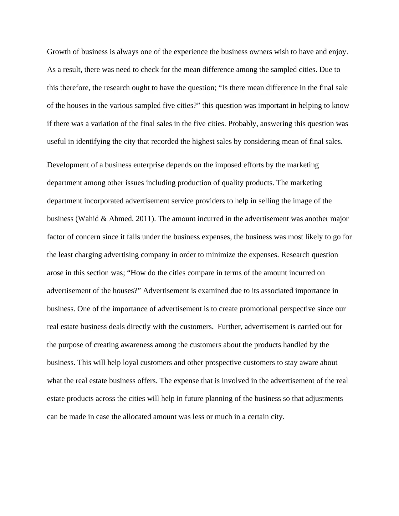
Growth of business is always one of the experience the business owners wish to have and enjoy.
As a result, there was need to check for the mean difference among the sampled cities. Due to
this therefore, the research ought to have the question; “Is there mean difference in the final sale
of the houses in the various sampled five cities?” this question was important in helping to know
if there was a variation of the final sales in the five cities. Probably, answering this question was
useful in identifying the city that recorded the highest sales by considering mean of final sales.
Development of a business enterprise depends on the imposed efforts by the marketing
department among other issues including production of quality products. The marketing
department incorporated advertisement service providers to help in selling the image of the
business (Wahid & Ahmed, 2011). The amount incurred in the advertisement was another major
factor of concern since it falls under the business expenses, the business was most likely to go for
the least charging advertising company in order to minimize the expenses. Research question
arose in this section was; “How do the cities compare in terms of the amount incurred on
advertisement of the houses?” Advertisement is examined due to its associated importance in
business. One of the importance of advertisement is to create promotional perspective since our
real estate business deals directly with the customers. Further, advertisement is carried out for
the purpose of creating awareness among the customers about the products handled by the
business. This will help loyal customers and other prospective customers to stay aware about
what the real estate business offers. The expense that is involved in the advertisement of the real
estate products across the cities will help in future planning of the business so that adjustments
can be made in case the allocated amount was less or much in a certain city.

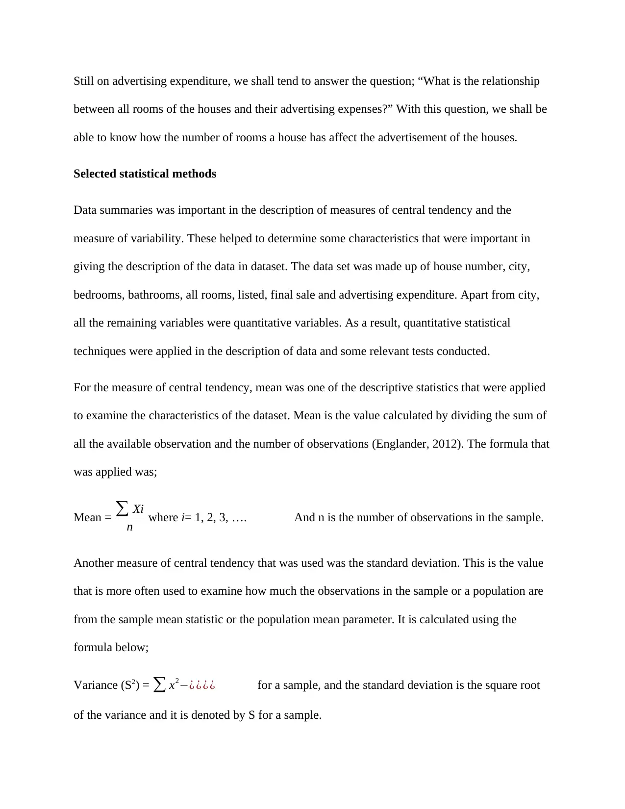
Still on advertising expenditure, we shall tend to answer the question; “What is the relationship
between all rooms of the houses and their advertising expenses?” With this question, we shall be
able to know how the number of rooms a house has affect the advertisement of the houses.
Selected statistical methods
Data summaries was important in the description of measures of central tendency and the
measure of variability. These helped to determine some characteristics that were important in
giving the description of the data in dataset. The data set was made up of house number, city,
bedrooms, bathrooms, all rooms, listed, final sale and advertising expenditure. Apart from city,
all the remaining variables were quantitative variables. As a result, quantitative statistical
techniques were applied in the description of data and some relevant tests conducted.
For the measure of central tendency, mean was one of the descriptive statistics that were applied
to examine the characteristics of the dataset. Mean is the value calculated by dividing the sum of
all the available observation and the number of observations (Englander, 2012). The formula that
was applied was;
Mean = ∑ Xi
n where i= 1, 2, 3, …. And n is the number of observations in the sample.
Another measure of central tendency that was used was the standard deviation. This is the value
that is more often used to examine how much the observations in the sample or a population are
from the sample mean statistic or the population mean parameter. It is calculated using the
formula below;
Variance (S2) = ∑ x2−¿ ¿ ¿ ¿ for a sample, and the standard deviation is the square root
of the variance and it is denoted by S for a sample.

S = √∑ x2−¿ ¿ ¿ ¿ ¿
In order to be able to identify the type of relationship that exist between variables, scatter plot
was used i.e. when determining the relationship type between all rooms variable and advertising
expenditure variable. The scatter plot was important to help in identification of whether the
relationship between the two variables was positive or negative. Also, the correlation coefficient
(r) was calculated,
r =n∑ xy−¿ ¿ ¿
Shape and symmetry of the data in the dataset was another issue of concern that resulted to the
incorporation of the box plot. This helped to show how data was distributed in the dataset for
various variables and whether or not there were outliers that would give deceptive information.
Requirement for the construction of the box plot, five point measures were required. They
included; the minimum, maximum, first quartile, median and third quartile (Ghasemi &
Zahediasl, 2012).
Mean of the final sales for various cities was an issue of concern that was also asked for in the
research questions. To solve this and have the question adequately answered, t-test was used and
therefore the hypothesis had to be formulated and tested otherwise. T-test was used to test for the
mean difference of the final sale for the five cities.
Technical analysis

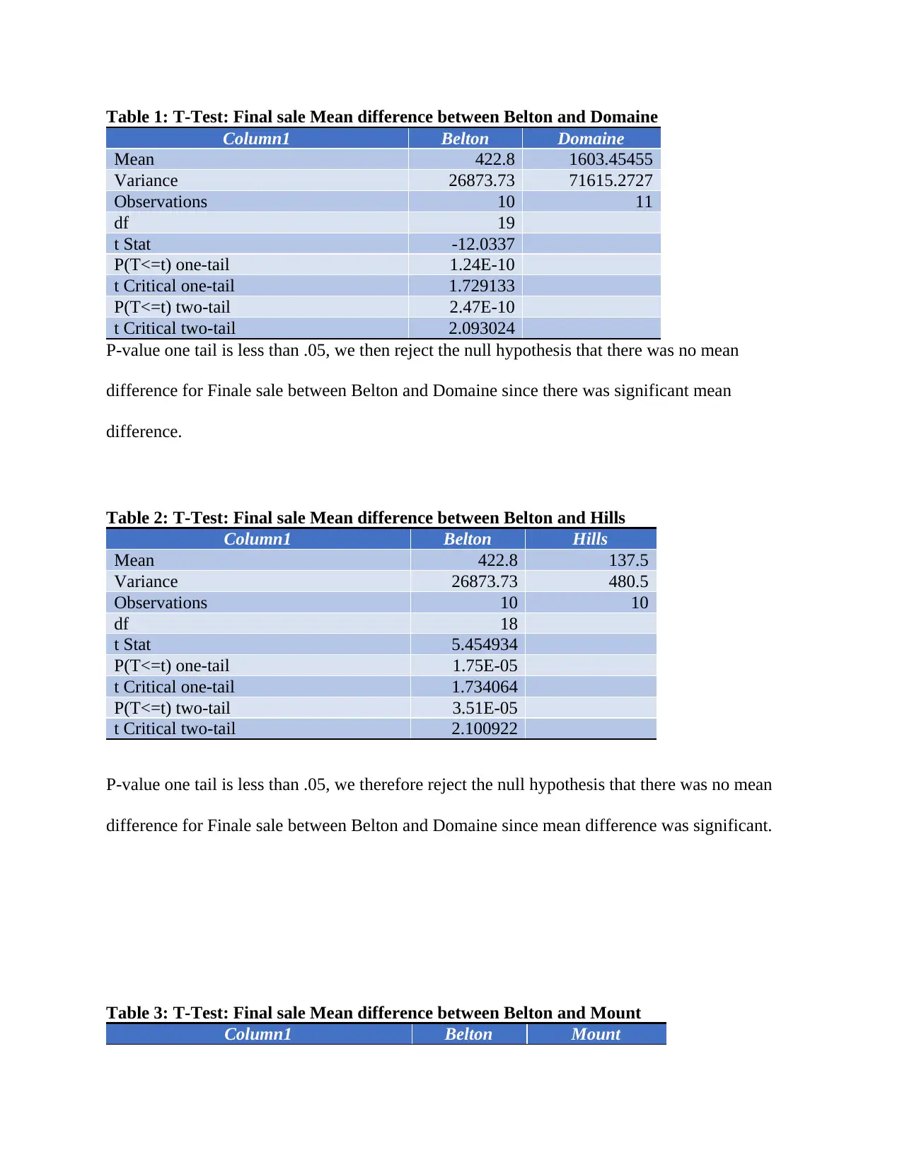
Table 1: T-Test: Final sale Mean difference between Belton and Domaine
Column1 Belton Domaine
Mean 422.8 1603.45455
Variance 26873.73 71615.2727
Observations 10 11
df 19
t Stat -12.0337
P(T<=t) one-tail 1.24E-10
t Critical one-tail 1.729133
P(T<=t) two-tail 2.47E-10
t Critical two-tail 2.093024
P-value one tail is less than .05, we then reject the null hypothesis that there was no mean
difference for Finale sale between Belton and Domaine since there was significant mean
difference.
Table 2: T-Test: Final sale Mean difference between Belton and Hills
Column1 Belton Hills
Mean 422.8 137.5
Variance 26873.73 480.5
Observations 10 10
df 18
t Stat 5.454934
P(T<=t) one-tail 1.75E-05
t Critical one-tail 1.734064
P(T<=t) two-tail 3.51E-05
t Critical two-tail 2.100922
P-value one tail is less than .05, we therefore reject the null hypothesis that there was no mean
difference for Finale sale between Belton and Domaine since mean difference was significant.
Table 3: T-Test: Final sale Mean difference between Belton and Mount
Column1 Belton Mount

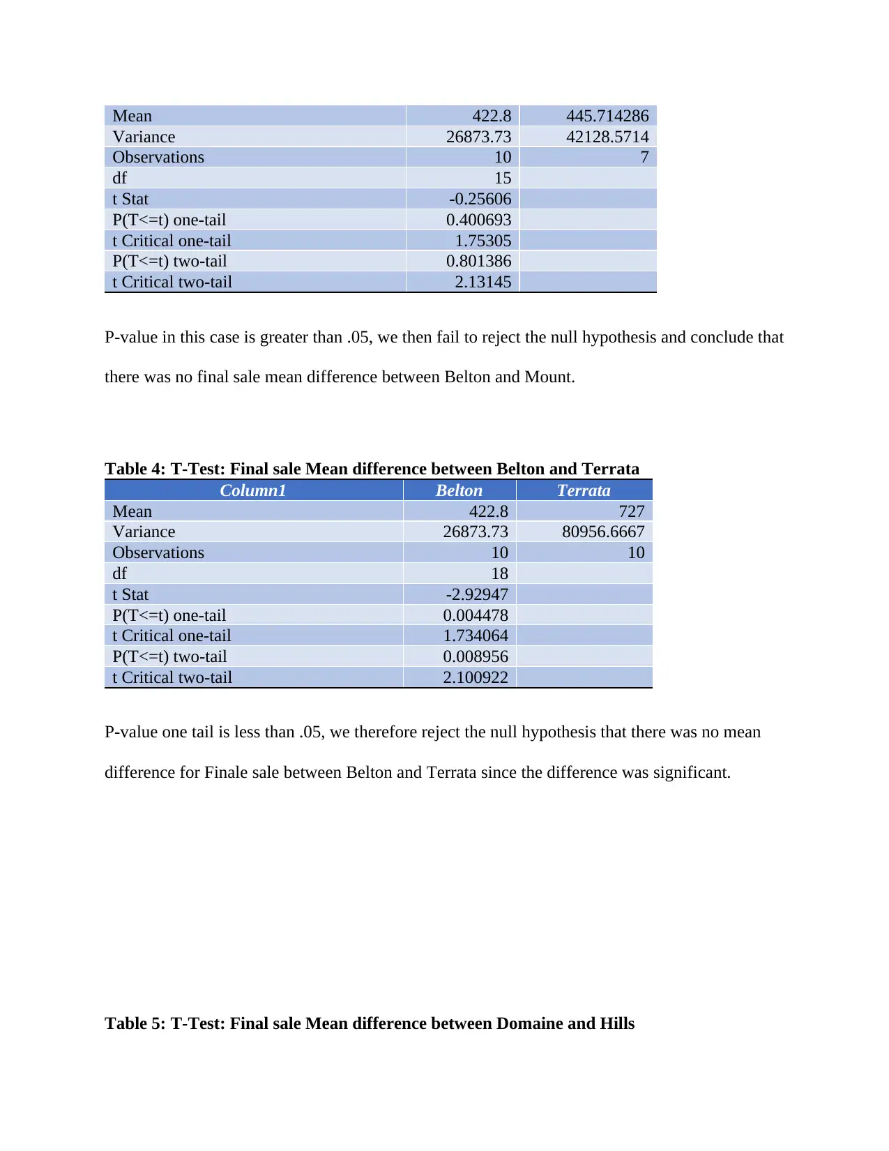
Mean 422.8 445.714286
Variance 26873.73 42128.5714
Observations 10 7
df 15
t Stat -0.25606
P(T<=t) one-tail 0.400693
t Critical one-tail 1.75305
P(T<=t) two-tail 0.801386
t Critical two-tail 2.13145
P-value in this case is greater than .05, we then fail to reject the null hypothesis and conclude that
there was no final sale mean difference between Belton and Mount.
Table 4: T-Test: Final sale Mean difference between Belton and Terrata
Column1 Belton Terrata
Mean 422.8 727
Variance 26873.73 80956.6667
Observations 10 10
df 18
t Stat -2.92947
P(T<=t) one-tail 0.004478
t Critical one-tail 1.734064
P(T<=t) two-tail 0.008956
t Critical two-tail 2.100922
P-value one tail is less than .05, we therefore reject the null hypothesis that there was no mean
difference for Finale sale between Belton and Terrata since the difference was significant.
Table 5: T-Test: Final sale Mean difference between Domaine and Hills

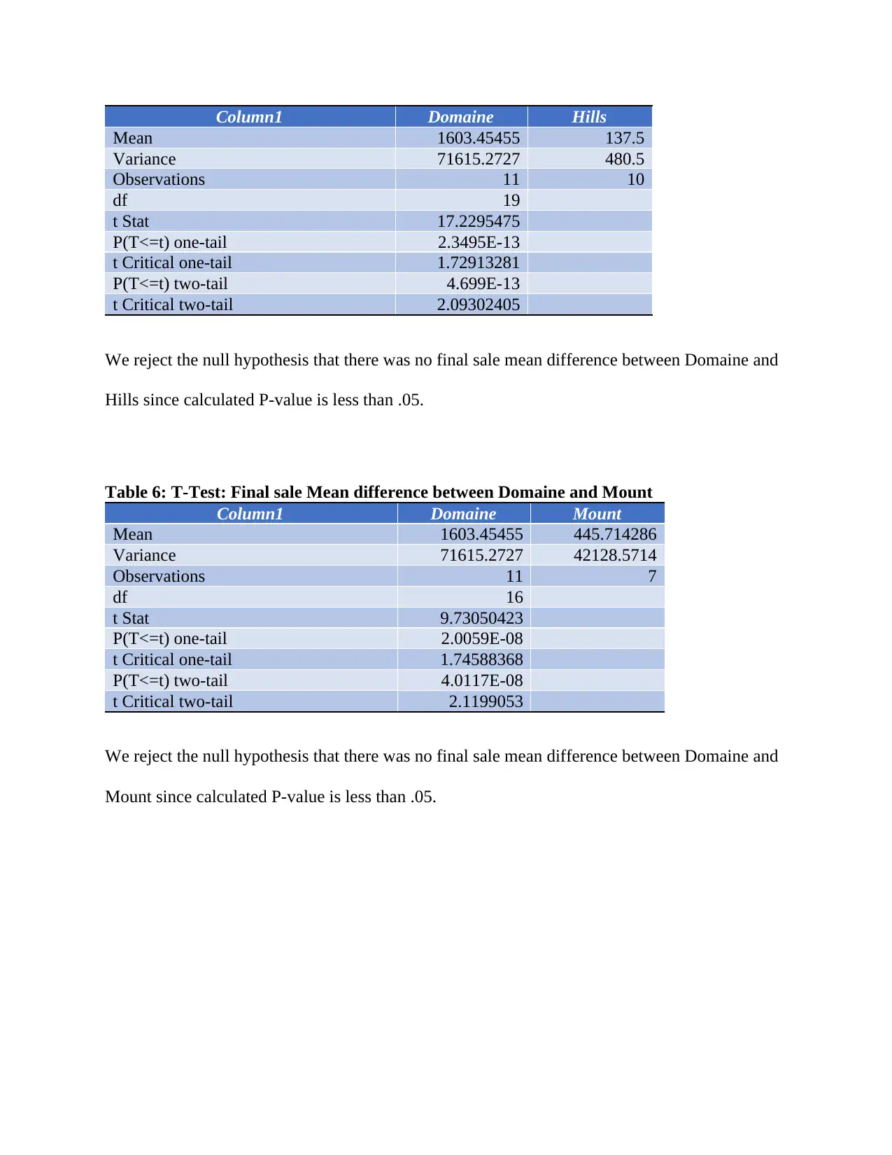
Column1 Domaine Hills
Mean 1603.45455 137.5
Variance 71615.2727 480.5
Observations 11 10
df 19
t Stat 17.2295475
P(T<=t) one-tail 2.3495E-13
t Critical one-tail 1.72913281
P(T<=t) two-tail 4.699E-13
t Critical two-tail 2.09302405
We reject the null hypothesis that there was no final sale mean difference between Domaine and
Hills since calculated P-value is less than .05.
Table 6: T-Test: Final sale Mean difference between Domaine and Mount
Column1 Domaine Mount
Mean 1603.45455 445.714286
Variance 71615.2727 42128.5714
Observations 11 7
df 16
t Stat 9.73050423
P(T<=t) one-tail 2.0059E-08
t Critical one-tail 1.74588368
P(T<=t) two-tail 4.0117E-08
t Critical two-tail 2.1199053
We reject the null hypothesis that there was no final sale mean difference between Domaine and
Mount since calculated P-value is less than .05.

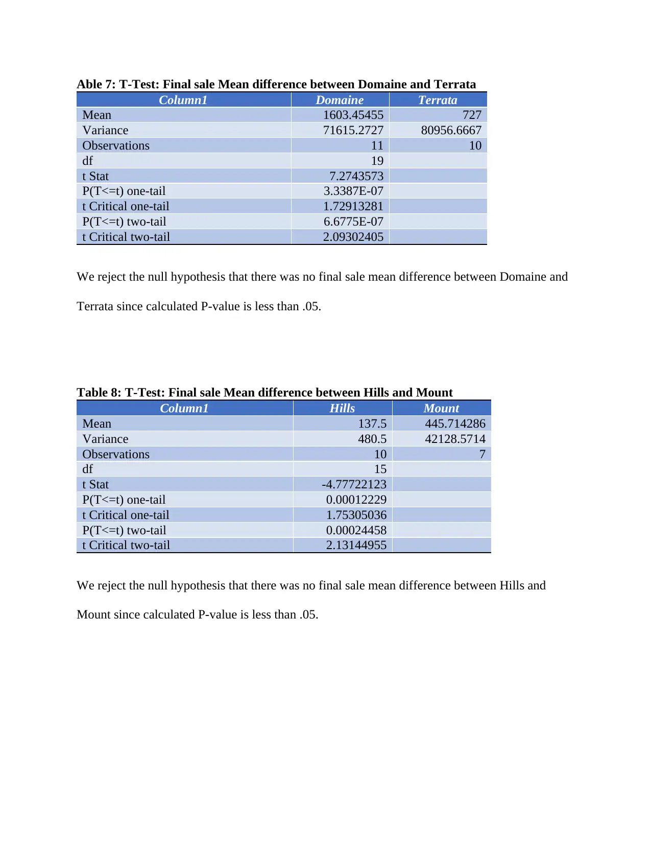
Able 7: T-Test: Final sale Mean difference between Domaine and Terrata
Column1 Domaine Terrata
Mean 1603.45455 727
Variance 71615.2727 80956.6667
Observations 11 10
df 19
t Stat 7.2743573
P(T<=t) one-tail 3.3387E-07
t Critical one-tail 1.72913281
P(T<=t) two-tail 6.6775E-07
t Critical two-tail 2.09302405
We reject the null hypothesis that there was no final sale mean difference between Domaine and
Terrata since calculated P-value is less than .05.
Table 8: T-Test: Final sale Mean difference between Hills and Mount
Column1 Hills Mount
Mean 137.5 445.714286
Variance 480.5 42128.5714
Observations 10 7
df 15
t Stat -4.77722123
P(T<=t) one-tail 0.00012229
t Critical one-tail 1.75305036
P(T<=t) two-tail 0.00024458
t Critical two-tail 2.13144955
We reject the null hypothesis that there was no final sale mean difference between Hills and
Mount since calculated P-value is less than .05.

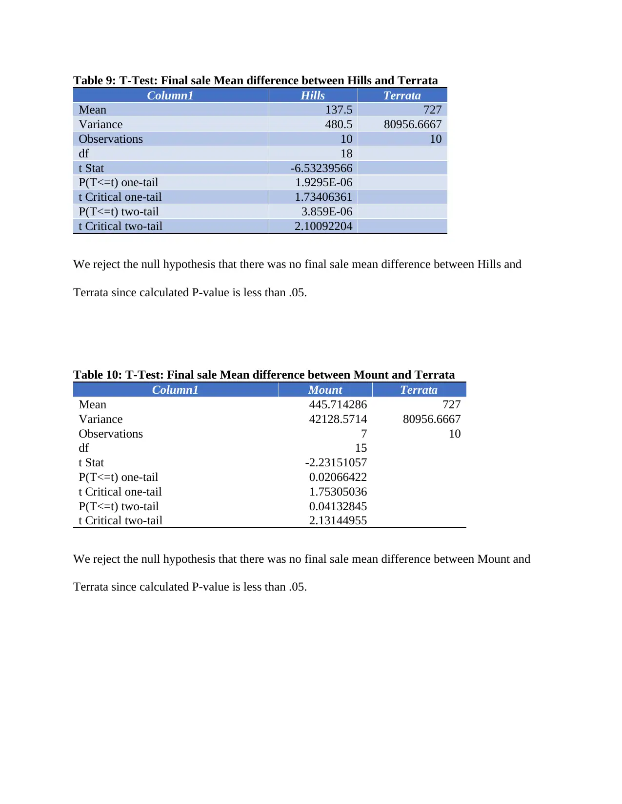
Table 9: T-Test: Final sale Mean difference between Hills and Terrata
Column1 Hills Terrata
Mean 137.5 727
Variance 480.5 80956.6667
Observations 10 10
df 18
t Stat -6.53239566
P(T<=t) one-tail 1.9295E-06
t Critical one-tail 1.73406361
P(T<=t) two-tail 3.859E-06
t Critical two-tail 2.10092204
We reject the null hypothesis that there was no final sale mean difference between Hills and
Terrata since calculated P-value is less than .05.
Table 10: T-Test: Final sale Mean difference between Mount and Terrata
Column1 Mount Terrata
Mean 445.714286 727
Variance 42128.5714 80956.6667
Observations 7 10
df 15
t Stat -2.23151057
P(T<=t) one-tail 0.02066422
t Critical one-tail 1.75305036
P(T<=t) two-tail 0.04132845
t Critical two-tail 2.13144955
We reject the null hypothesis that there was no final sale mean difference between Mount and
Terrata since calculated P-value is less than .05.

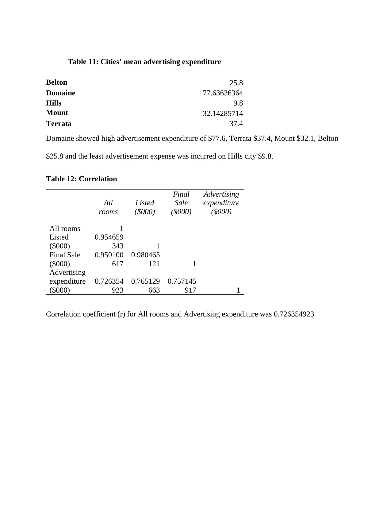
Domaine showed high advertisement expenditure of $77.6, Terrata $37.4, Mount $32.1, Belton
$25.8 and the least advertisement expense was incurred on Hills city $9.8.
Table 12: Correlation
All
rooms
Listed
($000)
Final
Sale
($000)
Advertising
expenditure
($000)
All rooms 1
Listed
($000)
0.954659
343 1
Final Sale
($000)
0.950100
617
0.980465
121 1
Advertising
expenditure
($000)
0.726354
923
0.765129
663
0.757145
917 1
Correlation coefficient (r) for All rooms and Advertising expenditure was 0.726354923
Table 11: Cities’ mean advertising expenditure
Belton 25.8
Domaine 77.63636364
Hills 9.8
Mount 32.14285714
Terrata 37.4

Figure 1: Scatter plot
0 5 10 15 20 25
0
20
40
60
80
100
120
140
R² = 0.527591473448742
Scatter plot for Advertising expenditure ($000)
against all rooms
All Rooms
Advertising expenditure ($000)
Coefficient of determination (R2) confirmed that the plots were 53% concentrated around the
trend line and there was strong positive correlation.

Figure 2: Box plot
Listed ($000) Final Sale ($000) Advertising expenditure
($000)
0
200
400
600
800
1000
1200
1400
1600
1800
2000
Q1 Median Q3
Listed values in the dataset were positively skewed as shown by box and whiskers above, final
sale was as well skewed to the right and lastly, advertising expenditure was also skewed to the
right showing that the data not normally distributed.
Results and discussions
T-tests were conducted to test for the final sale mean difference between various cities as
sampled. Through the tests, we had the first question answered. In regard to that therefore, we
would conclude that most cities showed final sale mean difference except for two towns i.e.
Belton and Mount that had their mean final sale too close to each other (422.8 and 445.714286)
that there was no significant difference could be detected by the test. From this therefore, the top
business officials are supposed to put different efforts to venture and maximize the profits from
those cities.

In response to the second question, mean advertising expenditure was calculated and Domaine
showed to have consumed the business a lot on advertisement as $77.6 was used. The amount
incurred on advertisement varied while we had some cities like Hills having the business
spending as low as $9.8. This variation can be considered to be as a result of internal or other
external factors of the business that were not determined by this research analysis.
The research was also interested in the relationship that would be existing between All rooms
variable and Advertising expenditure. To determine the type of relationship, correlation analysis
was conducted that revealed that there was strong positive correlation between the two variables
since the correlation coefficient (r) was 0.726354923. The relationship is shown in the scatter
plot above where its strength is at 53% as given by R-squared. The relationship meant that more
number of rooms a house has as indicated in all rooms will have an equally higher advertisement
expense incurred and when there are less rooms, low expenses will be incurred on
advertisements.
Tested variables from the sample showed that the data in the dataset were not normally
distributed but skewed. All variables that were plotted in the box and whisker showed that they
were all skewed to the right hand side thus positively skewed.

Reference
Abatecola, G., Caputo, A., Mari, M., & Poggesi, S. (2013). Real estate management: past,
present, and future research directions. International Journal of Globalisation and Small
Business, 5(1-2), 98-113.
Brounen, D., & de Koning, S. (2013). 50 years of real estate investment trusts: an international
examination of the rise and performance of REITs. Journal of Real Estate
Literature, 20(2), 197-223.
Cherif, E., & Grant, D. (2014). Analysis of e-business models in real estate. Electronic
Commerce Research, 14(1), 25-50.
Englander, M. (2012). The interview: Data collection in descriptive phenomenological human
scientific research. Journal of Phenomenological Psychology, 43(1), 13-35.
Ghasemi, A., & Zahediasl, S. (2012). Normality tests for statistical analysis: a guide for non-
statisticians. International journal of endocrinology and metabolism, 10(2), 486.
Lieser, K., & Groh, A. P. (2014). The determinants of international commercial real estate
investment. The Journal of Real Estate Finance and Economics,48(4), 611-659.
Soroca, A., & Karasic, N. J. (2012). U.S. Patent No. 8,302,030. Washington, DC: U.S. Patent
and Trademark Office.
Wahid, N. A., & Ahmed, M. (2011). The effect of attitude toward advertisement on Yemeni
female consumers' attitude toward brand and purchase intention. Global Business and
Management Research, 3(1), 21.

Appendix: Hypothesis
H0: there was no mean final sale difference among the sampled cities.
H1: There was mean final sale difference among the sampled cities