Real Estate Data Analysis Report: Price Prediction and Adv Spending

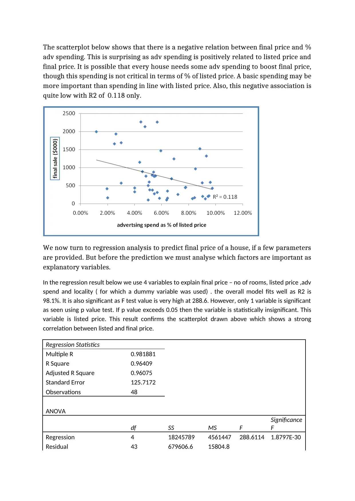
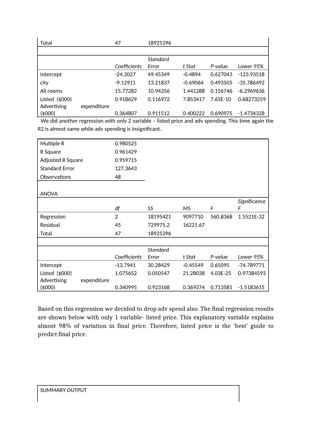
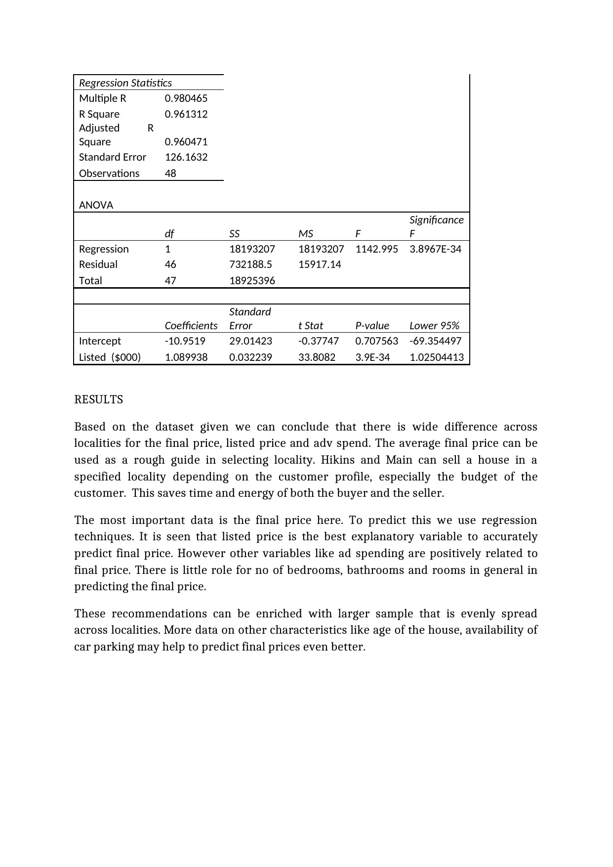
This report analyzes a dataset of 48 houses across different localities to address key research questions for real estate investment. The analysis employs statistical methods like measures of central tendency, dispersion, scatterplots, and regression techniques using Excel. The report investigates average house prices by locality, the impact of advertising spending on final prices, the relationship between listed and final prices, and predictive modeling for final prices. Key findings include the highest prices in Domaine, a positive correlation between advertising spend and final price (though moderate), and a strong positive association between listed and final prices. Regression analysis reveals that listed price is the most significant predictor of final price, explaining approximately 98% of the variation. The report concludes with recommendations for investors, emphasizing the importance of listed price in predicting final sale price and suggesting the need for a larger, more evenly distributed sample size for further analysis.

Cover sheet

INTRODUCTION
This report is based on a sample of 48 observations of houses in different localities,
along with data on the no of rooms, bedrooms, bathrooms, listed price, final price and
adv spend on each house. We use this data to answer research questions outlined
below, and use graphs/visual aids to present the data in easier ways for interpretation.
Hopefully, Hikins & Main will be able to use this analysis for their investments in the future in real
estate sector.
RESEARCH QUESTIONS
We can look at this data to answer the following questions:
We gauge the average price of a house in each locality. This serves as a rough guide for
prospective buyers in terms of which area to consider, depending on their budget for
the house.
What should be the adv spending on a house so that such spending fetches a higher final
price. This will help sellers to decide if adv is worth the money, and returns from selling
compensate the adv spending.
How closely are listed and final price associated? If there is a close positive relation then
it may help sellers to set a higher fixed price, in hopes of a higher final price.
Can we predict the final price of a house using some variables given to us? We attempt
to find variables that can explain the variation in final price of a house. We ask if more
bedrooms lead to a higher price or if higher adv spends can increase price at which a
house is sold.
SELECTED STATISTICAL METHODS
We will use Excel for this report and report on data given with the use of following
statistical methods:
 Measures of central tendency -mean and median
 Measures of dispersion
 Scatterplots
 Regression techniques

 Bar charts
TECHNICAL ANALYSIS
Note that the share of 5 localities is not even in the sample as seen below. Domaine has most no of
houses while Mount has least.
City
Belton Domaine Hills Mount Terratae
10 11 10 7 10
Next, we look at the average list and final price for each house, along with the % adv spend. This is
calculated as 100*adv spending/ final price. The table below shows that average final price is
$752710, while average listed price is $700650. The average adv spend is 6.22% of final price. All
three are positively skewed which implies that most houses lie at lower end of the range of values.
listed P final P
% ad
spend
Mean 700.65 752.71 6.22
Standard Error 82.39 91.59 0.36
Median 500.00 535.00 5.96
Mode 400.00 101.00 #N/A
Standard
Deviation 570.83 634.56 2.49
Sample Variance 325842.83 402668.00 6.19
Kurtosis -0.51 0.14 -0.11
Skewness 0.92 1.11 0.24
Note that a simple average across localities can be misleading as we have different
samples in each locality. The next chart shows average prices locality wise for better
understanding.

Clearly prices are highest in Domaine, while they are lowest in Hills. This chart allows
buyers to pick and choose a locality to shop in, depending on their budget.
The adv spending follows a similar pattern in each locality as shown below. An average
of $77600 is spent on each house as compared to only $9800 in Hills.
Domaine stands out as the most expensive locality on all three parameters.

We look at the role of advertising on prices now. The scatterplot below shows that
higher is adv spend greater is final price. This positive association signals that sellers
must spend on adv. But the strength of this association is only moderate as shown by
the value of R2 = 0.573. This implies that only 57.3% of variation in listed price is
explained by variation in adv spending.
We also see a strong positive association between final and listed price as seen below.
This association is very strong – higher is the listed price higher is final price. The R2
value is extremely high at 0.961. This implies that 96.1% of variation in final price is
explained by variation in listed price. If sellers can get a good listed price they have high
chances of getting a high final price as well.
We now ask ourselves how much adv spending is recommended, since it is positively
associated with final price. We use a new variable- adv spending as a % of listed price.

The scatterplot below shows that there is a negative relation between final price and %
adv spending. This is surprising as adv spending is positively related to listed price and
final price. It is possible that every house needs some adv spending to boost final price,
though this spending is not critical in terms of % of listed price. A basic spending may be
more important than spending in line with listed price. Also, this negative association is
quite low with R2 of 0.118 only.
We now turn to regression analysis to predict final price of a house, if a few parameters
are provided. But before the prediction we must analyse which factors are important as
explanatory variables.
In the regression result below we use 4 variables to explain final price – no of rooms, listed price ,adv
spend and locality ( for which a dummy variable was used) . the overall model fits well as R2 is
98.1%. It is also significant as F test value is very high at 288.6. However, only 1 variable is significant
as seen using p value test. If p value exceeds 0.05 then the variable is statistically insignificant. This
variable is listed price. This result confirms the scatterplot drawn above which shows a strong
correlation between listed and final price.
Regression Statistics
Multiple R 0.981881
R Square 0.96409
Adjusted R Square 0.96075
Standard Error 125.7172
Observations 48
ANOVA
df SS MS F
Significance
F
Regression 4 18245789 4561447 288.6114 1.8797E-30
Residual 43 679606.6 15804.8

Total 47 18925396
Coefficients
Standard
Error t Stat P-value Lower 95%
Intercept -24.2027 49.45349 -0.4894 0.627043 -123.93518
city -9.12911 13.21837 -0.69064 0.493505 -35.786492
All rooms 15.77282 10.94356 1.441288 0.156746 -6.2969636
Listed ($000) 0.918629 0.116972 7.853417 7.65E-10 0.68273259
Advertising expenditure
($000) 0.364807 0.911512 0.400222 0.690975 -1.4734328
We did another regression with only 2 variable – listed price and adv spending. This time again the
R2 is almost same while adv spending is insignificant.
Multiple R 0.980525
R Square 0.961429
Adjusted R Square 0.959715
Standard Error 127.3643
Observations 48
ANOVA
df SS MS F
Significance
F
Regression 2 18195421 9097710 560.8368 1.5521E-32
Residual 45 729975.2 16221.67
Total 47 18925396
Coefficients
Standard
Error t Stat P-value Lower 95%
Intercept -13.7941 30.28429 -0.45549 0.65095 -74.789771
Listed ($000) 1.075652 0.050547 21.28038 4.03E-25 0.97384593
Advertising expenditure
($000) 0.340995 0.923168 0.369374 0.713581 -1.5183615
Based on this regression we decided to drop adv spend also. The final regression results
are shown below with only 1 variable- listed price. This explanatory variable explains
almost 98% of variation in final price. Therefore, listed price is the ‘best’ guide to
predict final price.
SUMMARY OUTPUT

Regression Statistics
Multiple R 0.980465
R Square 0.961312
Adjusted R
Square 0.960471
Standard Error 126.1632
Observations 48
ANOVA
df SS MS F
Significance
F
Regression 1 18193207 18193207 1142.995 3.8967E-34
Residual 46 732188.5 15917.14
Total 47 18925396
Coefficients
Standard
Error t Stat P-value Lower 95%
Intercept -10.9519 29.01423 -0.37747 0.707563 -69.354497
Listed ($000) 1.089938 0.032239 33.8082 3.9E-34 1.02504413
RESULTS
Based on the dataset given we can conclude that there is wide difference across
localities for the final price, listed price and adv spend. The average final price can be
used as a rough guide in selecting locality. Hikins and Main can sell a house in a
specified locality depending on the customer profile, especially the budget of the
customer. This saves time and energy of both the buyer and the seller.
The most important data is the final price here. To predict this we use regression
techniques. It is seen that listed price is the best explanatory variable to accurately
predict final price. However other variables like ad spending are positively related to
final price. There is little role for no of bedrooms, bathrooms and rooms in general in
predicting the final price.
These recommendations can be enriched with larger sample that is evenly spread
across localities. More data on other characteristics like age of the house, availability of
car parking may help to predict final prices even better.

Anon., n.d. Mean, median, mode. [Online] Available at:
http://www.bbc.co.uk/schools/gcsebitesize/maths/statistics/measuresofaveragerev6.shtml
[Accessed 18 Sep 2017].
Dizikes, P., 2010. news.mit.edu. [Online] (http://news.mit.edu/2010/explained-reg-analysis-0316)
[Accessed 19 Sep 2017].
Home.iitk.ac.in, n.d. Regression analysis. [Online] Available atSimpleLinearRegressionAnalysis.pdf"
http://home.iitk.ac.in/~shalab/regression/Chapter2-Regression-SimpleLinearRegressionAnalysis.pdf
[Accessed 16 SEp 2017].
Manikandan, S., 2011. Mesures of central tendenecy. Journal of Pharmacology, 2(3), pp.214-15.
Marley, S., n.d. Imprtance and effect of sample size. [Online] Available at: https://select-
statistics.co.uk/blog/importance-effect-sample-size/ [Accessed 17 Sep 2017].
Rgs.org, n.d. Sampling techniques. [Online] Available at:
http://www.rgs.org/OurWork/Schools/Fieldwork+and+local+learning/Fieldwork+techniques/
Sampling+techniques.htm [Accessed 18 June 2017].
stat.ualberta.ca, n.d. What isa P value. [Online] Available at:
http://www.stat.ualberta.ca/~hooper/teaching/misc/Pvalue.pdf [Accessed 19 Sep 2017].