Real Estate Market Analysis Report for State A Residential Properties

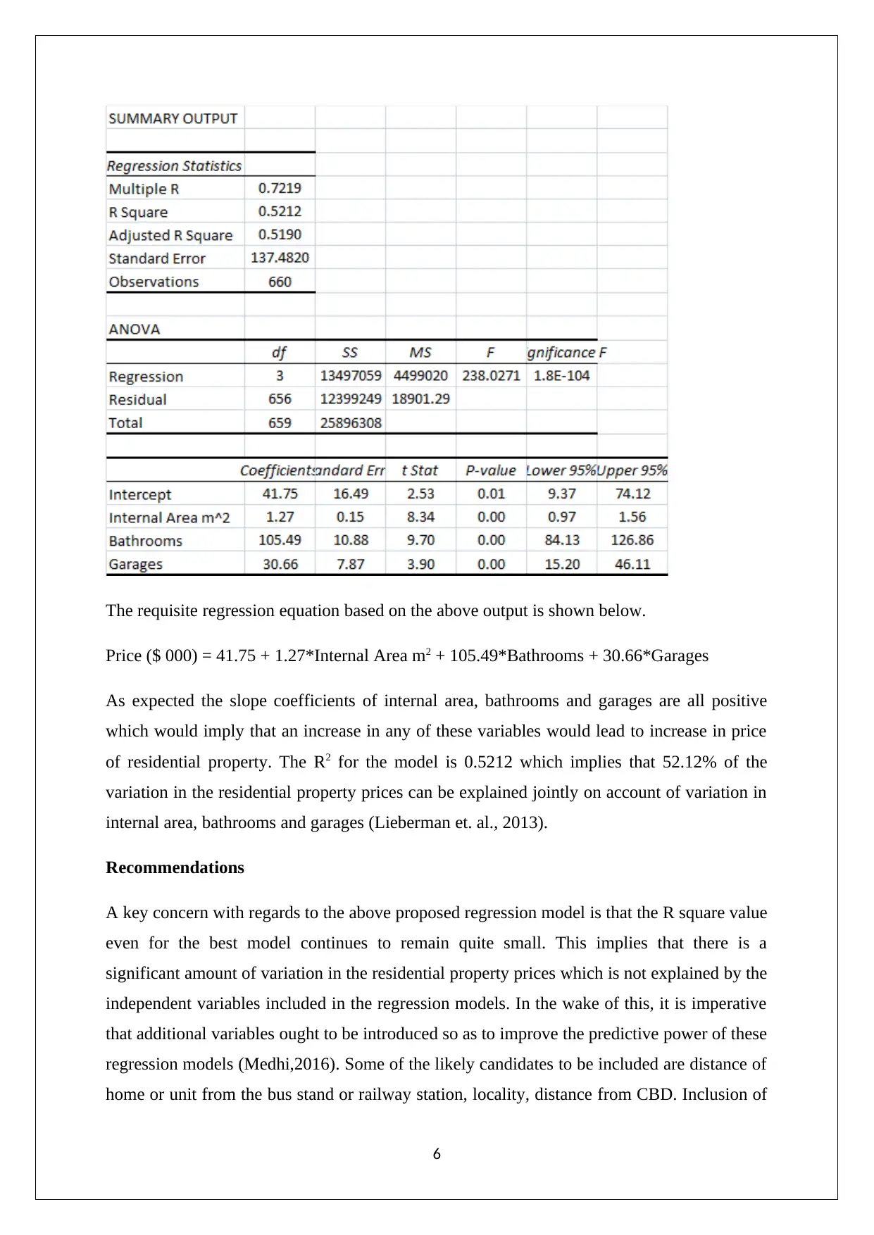
This report presents an analysis of the real estate market in non-capital cities and towns within State A, focusing on predicting residential property prices. The study employs descriptive statistics to understand the characteristics of properties across regional cities, coastal cities, and coastal towns. A multiple regression model is developed to estimate house prices, considering variables such as internal area, number of bathrooms, and garages. The findings reveal that internal area, bathrooms, and garages have a positive impact on property prices. However, the model's R-squared value indicates that there is still a significant amount of variation in property prices not explained by the included variables, suggesting that the model can be improved by including additional variables. The report recommends incorporating factors such as the distance to public transport and CBD. The report also notes that the type of property (house or unit) does not significantly influence the price. The analysis is based on data provided by Safe-As-House Real Estate and adheres to the guidelines of the Business Analytics and Big Data (ACC73002) assignment.

DATA ANALYTICS
STUDENT ID:
[Pick the date]

Introduction and Background
During the last decade or so, property prices in Australia have soared which is particularly
true for certain cities such as Sydney and Melbourne. As a result, the investment in real
estate has seen a significant increase in the last two decades or so. It is essential to determine
a intrinsic value of various residential properties so that the clients can be advised with
regards to a fair price for a given property. In this backdrop, the objective of the given report
is to predict the fair value of the residential property prices in non-capital cities and towns
corresponding to State A. In this regards, data has been provided from the relevant cities and
towns which corresponds to data about the houses which have been recently sold.
Data and Empirical Strategy
Sample data has been presented in order to facilitate the summary of data and also estimation
of best multiple regression model to estimate the prices for the various residential properties
(i.e. house and unit) based on their relevant attributes. The starting point is the data which
has been segregated for the coastal city, coastal town along with regional city. The underlying
objective is to produce the best possible multiple regression model for the estimation of
residential property. The data sample includes information about various variables such as
price, internal area, number of bedrooms, number of garages, number of bathrooms. Further,
there are certain variables such as Land area for which data is available only in particular
cities and not available for all properties. Most of the variables are quantitative in nature and
measures based on ratio scale since there is an absolute zero which can be defined as
variables such as price, number of bedrooms, bathrooms, garages cannot assume negative
values. A key example of categorical variable is type which has been measured using
nominal scale since two possible labels namely unit and house are possible (Flick, 2015).
The first step in data analysis is to compute the descriptive statistics for the various
quantitative variables which provides a summary of these based on regional city, coastal city
and town. In order to understand any differences in the sample with regard to price of other
attributes, a comparison of the descriptive statistics in accordance with the location has been
carried. With regards to the estimation of the regression model, the cumulative data for state
A has been considered. Some variables are available for only properties located in a
particular city or town. These variables have not been taken into consideration for the
multiple regression thereby limiting the participation of only those variables which are
available for all properties included in the sample.
2

The first step is to run the multiple regression model with the aid of MS-Excel where price
would act as the dependent variable and all the various variables for which data on all
properties is available would serve as independent variables. The tweaking of this model
would be performed based on the statistical significance of the respective slopes of the
independent variables used for the regression model. The independent variables which are
found to be statistically insignificant would be ignored and the multiple regression would be
run without these variables so as to enhance the statistical significance of the regression
model (Hair et. al., 2015).
Results and Discussion
The descriptive statistics for the residential properties to regional city in state A are
summarised below.
The descriptive statistics for the residential properties to coastal city in state A are
summarised below.
3

The descriptive statistics for the residential properties to coastal town in state A are
summarised below.
The objective is to draw a comparison between the descriptive statistics in three different
locations in state A. This is carried below.
Price: A common feature for price across the three locations is the existence of high skew
owing to which the average price would be best captured by median rather than mean
(Eriksson and Kovalainen, 2015). Comparing the median prices across the three locations, it
is evident that the prices are lowest for regional city while maximum for coastal town.
Further, the extent of dispersion in the price also seems to be influenced by the median prices
as more volatility is observed in locations exhibiting higher median prices.
Internal Area: Owing to presence of skew, it would be preferable to compare the median
value. There does not seem to be any significant difference in the median internal area across
the three types of locations in State A. The median area is marginally lower for coastal city.
Also, the extent of dispersion in this variables does not significant differ across the three
locations in state A (Hair et. al., 2015).
Bedrooms: The median value of bedrooms for the sample data across the three locations in
state A is the same at 3 bedrooms. This implies that for all the three locations, there ar e 50%
properties in the sample data where the bedrooms do not exceed 3. The extent of dispersion
in the number of bedrooms for the three locations also does not show any meaning difference
to be of any statistical significance.
Bathrooms: The median bathrooms for properties located in coastal city and town is 2 while
that for properties located in regional city, it is 1. This suggests that in regional city, half of
the sample properties would not have more than 1 bathrooms (Hillier, 2016). In terms of
4

variation, lesser variation is observed for this variable in the regional city as compared to the
coastal city and town.
Garages: Owing to highly skewed nature of this variable, the median is compared across
locations in state A. it has been seen that median garages is 1 for sample properties in coastal
city while the corresponding value is 2 for sample properties at other two locations namely
coastal town and regional city. The extent of dispersion in the given variable does not differ
significantly across the three locations.
Estimation of multiple regression
In order to frame a multiple linear regression model for the estimation for the residential
properties, the dependent variable has been taken as price while the independent variables to
begin with were internal area, bedroom, garage, bathroom along with type of unit. In order to
capture the potential influence of type of residential property on the price, a 0/1 notation has
been used whereby unit has been represented by 0 and a house by 1. The initial multiple
regression with all the above variables as independent variables indicated that the influence
of type on price was not statistically significant and hence this independent variables was
removed from the regression model. Also, the slope corresponding to number of bedrooms
was also not significant thereby implying that the bedroom count did not materially influence
the price (Taylor and Cihon, 2017). As a result, the final multiple regression model has been
proposed with three independent variables namely the internal area, bathroom and garages.
The requisite output obtained from the regression analysis using MS-Excel is indicated as
follows.
5

The requisite regression equation based on the above output is shown below.
Price ($ 000) = 41.75 + 1.27*Internal Area m2 + 105.49*Bathrooms + 30.66*Garages
As expected the slope coefficients of internal area, bathrooms and garages are all positive
which would imply that an increase in any of these variables would lead to increase in price
of residential property. The R2 for the model is 0.5212 which implies that 52.12% of the
variation in the residential property prices can be explained jointly on account of variation in
internal area, bathrooms and garages (Lieberman et. al., 2013).
Recommendations
A key concern with regards to the above proposed regression model is that the R square value
even for the best model continues to remain quite small. This implies that there is a
significant amount of variation in the residential property prices which is not explained by the
independent variables included in the regression models. In the wake of this, it is imperative
that additional variables ought to be introduced so as to improve the predictive power of these
regression models (Medhi,2016). Some of the likely candidates to be included are distance of
home or unit from the bus stand or railway station, locality, distance from CBD. Inclusion of
6

more independent variables could improve the results. Also, it is seen that price of the preprty
is independent of the underlying type (i.e. house and unit) and thereby the same may be
ignored. More research ought to be performed regarding the same so as to enhance the
understanding of property market in state A (Lind, Marchal and Wathen, 2014).
7

References
Eriksson, P. and Kovalainen, A. (2015) Quantitative methods in business research. 3rd ed.
London: Sage Publications.
Flick, U. (2015) Introducing research methodology: A beginner's guide to doing a research
project. 4th ed. New York: Sage Publications.
Hair, J. F., Wolfinbarger, M., Money, A. H., Samouel, P., and Page, M. J. (2015) Essentials
of business research methods. 2nd ed. New York: Routledge.
Hastie, T., Tibshirani, R. and Friedman, J. (2014) The Elements of Statistical Learning. 4th
ed. New York: Springer Publications.
Hillier, F. (2016) Introduction to Operations Research.6th ed.New York: McGraw Hill
Publications.
Lieberman, F. J., Nag, B., Hiller, F.S. and Basu, P. (2013) Introduction To Operations
Research. 5th ed.New Delhi: Tata McGraw Hill Publishers.
Lind, A.D., Marchal, G.W. and Wathen, A.S. (2014) Statistical Techniques in Business and
Economics. 15th ed. New York : McGraw-Hill/Irwin.
Medhi, J. (2016) Statistical Methods: An Introductory Text. 4th ed. Sydney: New Age
International.
Taylor, K. J. and Cihon, C. (2017) Statistical Techniques for Data Analysis. 2nd ed.
Melbourne: CRC Press.
8