Regression Analysis of Real Estate Pricing Determinants in Australia

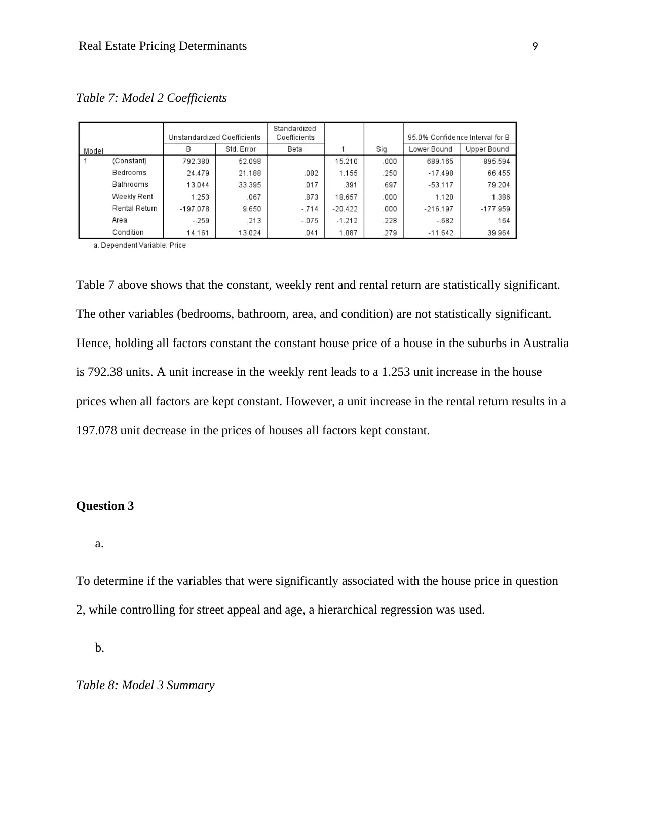
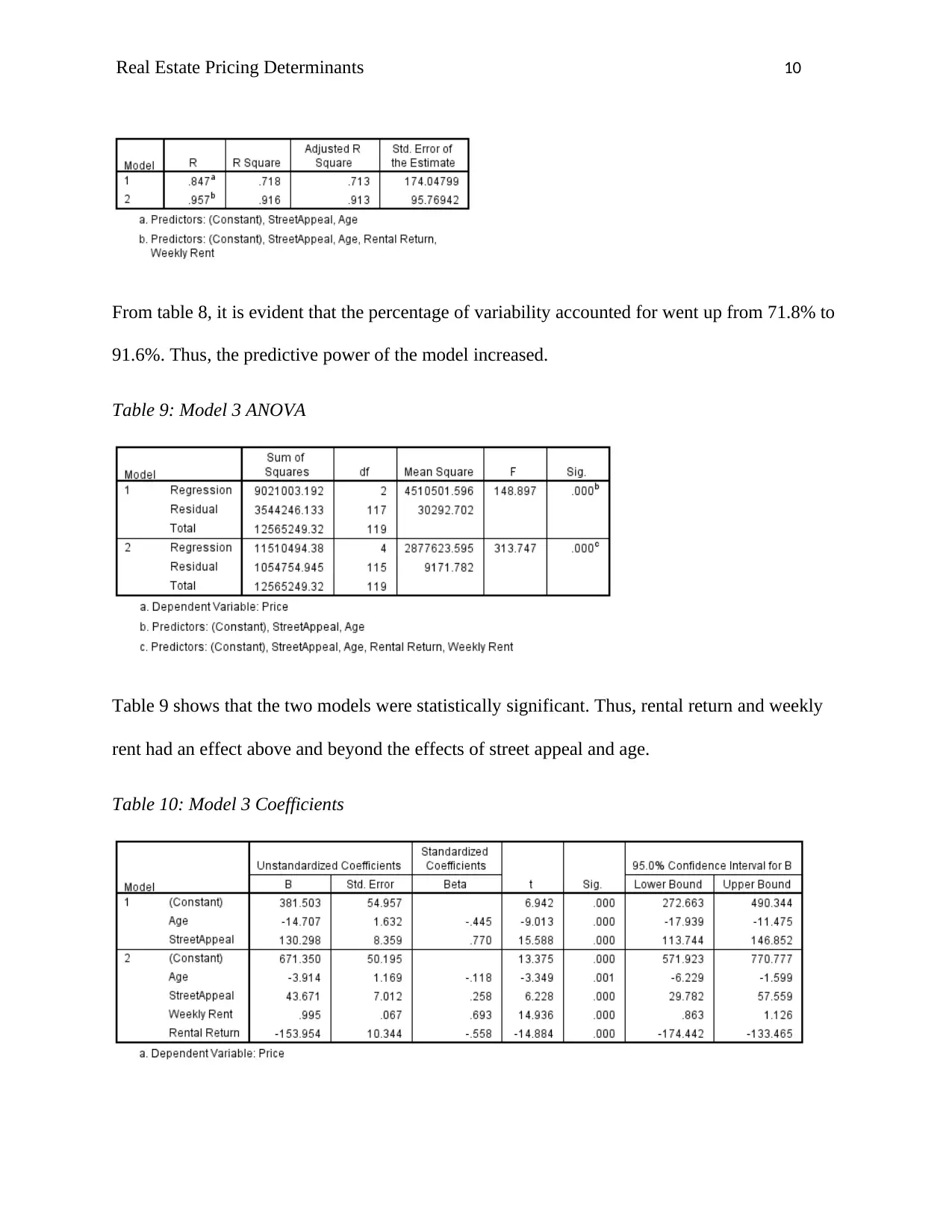
This report presents a comprehensive analysis of real estate pricing determinants using various regression models. The study begins with a linear regression to determine the predictive power of weekly rent on house prices, confirming a statistically significant relationship where a unit increase in weekly rent leads to a corresponding increase in house price. Subsequently, a multiple regression model is employed to evaluate the impact of multiple variables, including the number of bedrooms, bathrooms, rental return, area, and condition of the house, revealing that weekly rent and rental return are statistically significant predictors. Finally, a hierarchical regression model is used to determine the variables significantly associated with house prices, while controlling for street appeal and age, enhancing the predictive power of the model. The report adheres to the assumptions of each regression model and provides detailed statistical results, including model summaries, ANOVA tables, and coefficients, to support the findings.

RUNNING HEADER: REAL ESTATE PRICING DETERMINANTS 1
Real Estate Pricing Determinants
Students name:
Students ID:
Institution:

Real Estate Pricing Determinants 2
Question 1
a.
To determine how well the weekly rent predicts the house price, a linear regression model will
be adopted. A linear regression model is the most appropriate in predicting the values of a
variable on the basis of another variable (Seber & Lee, 2012). In this case, the house price is the
dependent variable while the weekly rent is the independent variable.
b.
Before carrying out a linear regression model, six assumptions have to be checked in order to
ensure that the data adhere to them. The assumptions include, the two variables measured should
be continuous, there should be a linear relationship between the two variables, there should be no
significant outliers, there is the independence of observations, there is homoscedasticity, and
residual of regression line are approximately normally distributed.
c.
The data can be shown to have met all the six assumptions. For starters, the two variables are
continuous in nature thereby meeting assumption 1. The second assumption can be seen in the
scatterplot below where it is seen that there is a linear relationship between the two variables.

Real Estate Pricing Determinants 3
Figure 1: Price against weekly rent scatterplot
Consequently, from figure 1 above, it can be seen that there are no significant outliers.
A Durbin-Watson test was carried out and the result was 1.541. Since the result is between 1.5
and 2.5, we can conclude that the data is not autocorrelated (Chatterjee & Haji, 2015). Thus,
there is the independence of observations. The assumption of homoscedasticity was also
confirmed since the derived VIF was 1. Since the value does not exceed 10, then it is safe to say
that there is no multicollinearity.
Figure 2: Histogram of residual of the regression
In figure 2 above, it is evident that the sixth assumption has been met since the residual of the
regression line is normally distributed.
d.
Table 1: Model 1 Summary

Real Estate Pricing Determinants 4
From table 1 above, it can be seen that the variable accounts for 43.8% of the variability in the
model. On the other hand, 56.2% of the variability is explained by variables, not in the model.
Table 2: Model 1 ANOVA
The model fits a straight line since it can be observed in table 2 above that the model is
statistically significant.
Table 3: Model 1 Coefficients
From the regression model in table 3 above, it can be seen that holding all factors constant, the
constant house price of a house in the suburb in Australia is 309.34 units. The constant is
statistically significant (p < 0.05). A unit increase in the weekly rent leads to a 0.955 unit

Real Estate Pricing Determinants 5
increase in the house price of a house in the suburb, holding all other factors constant. The
coefficient can also be seen to be statistically significant (p < 0.05).
Thus, the weekly rent predicts the house price where a unit increase in weekly rent leads to a
0.955 unit increase in house price. The model is statistically significant as weekly rent accounts
for 43.8% of the changes in house price in Australia suburbs.
Question 2
a.
To determine if the house price is predicted by the number of bedrooms, a number of bathrooms,
weekly rent, rental return, area and condition of the house, a multiple regression will be used.
The method is the most suitable since it predicts the value of a variable on the basis of the value
of two or more other variables (Cohen, West & Aiken 2014).
b.
A multiple regression has eight assumptions (Keith, 2012). The first assumption is that the
dependent variable is continuous. The other assumptions are that there are two or more
independent variables which can either be continuous or ordinal, there is the independence of
observations, there is a linear relationship between the dependent and each independent
variables, data must show multicollinearity, there are no significant outliers and the residuals are
approximately normally distributed.
c.
The data did not meet all the eight afro-mentioned assumptions. The first assumption was met
since the dependent variable, house price is continuous. There were more than one independent

Real Estate Pricing Determinants 6
variables; the number of bedrooms, number of bathrooms, weekly rent, rental return, area and
condition of the house which are either continuous or ordinal. A Durbin-Watson test was carried
out and the result was 1.784. Since the result is between 1.5 and 2.5, we can conclude that the
data is not autocorrelated. Thus, there is the independence of observations. Consequently, it was
seen that there was a linear relationship between the dependent and each independent variables
as seen in the figures below.

Real Estate Pricing Determinants 7
From the above figures, it can, however, be seen that there are outliers in some of the variables
such as area, condition, number of bathrooms, and number of bedrooms. The table below shows
the VIF of the independent variables.
Table 4: VIF
Variables VIF
Bedrooms 5.260
Bathrooms 1.922
Weekly Rent 2.284
Rental Return 1.275
Area 3.987
Condition 1.471
The VIF of the variables can be seen to be less than 10, thus, there is no multicollinearity. The
final assumption was confirmed to be met since from figure 3 below shows that the regression
residuals are normally distributed.

Real Estate Pricing Determinants 8
Figure 3: Histogram of residual of the regression
d.
Table 5: Model 2 summary
Table 5 shows that the variables account for 88.6% of the variability in the model. On the other
hand, 11.4% of the variability is explained by variables not in the model.
Table 6: Model 2 ANOVA
The model fits a straight line since it can be observed in table 6 above that the model is
statistically significant.

Real Estate Pricing Determinants 9
Table 7: Model 2 Coefficients
Table 7 above shows that the constant, weekly rent and rental return are statistically significant.
The other variables (bedrooms, bathroom, area, and condition) are not statistically significant.
Hence, holding all factors constant the constant house price of a house in the suburbs in Australia
is 792.38 units. A unit increase in the weekly rent leads to a 1.253 unit increase in the house
prices when all factors are kept constant. However, a unit increase in the rental return results in a
197.078 unit decrease in the prices of houses all factors kept constant.
Question 3
a.
To determine if the variables that were significantly associated with the house price in question
2, while controlling for street appeal and age, a hierarchical regression was used.
b.
Table 8: Model 3 Summary

Real Estate Pricing Determinants 10
From table 8, it is evident that the percentage of variability accounted for went up from 71.8% to
91.6%. Thus, the predictive power of the model increased.
Table 9: Model 3 ANOVA
Table 9 shows that the two models were statistically significant. Thus, rental return and weekly
rent had an effect above and beyond the effects of street appeal and age.
Table 10: Model 3 Coefficients

Real Estate Pricing Determinants 11
All the predictors in this model were found to be statistically significant. Thus, the betas can be
used as the weights which can be used as scores to be multiplied on the independent variables so
as to get predicted the score of a housing price on the dependent variable.

Real Estate Pricing Determinants 12
References:
Chatterjee, S., & Hadi, A. S. (2015). Regression analysis by example. John Wiley & Sons.
Cohen, P., West, S. G., & Aiken, L. S. (2014). Applied multiple regression/correlation analysis
for the behavioral sciences. Psychology Press.
Keith, T. Z. (2014). Multiple regression and beyond: An introduction to multiple regression and
structural equation modeling. Routledge.
Seber, G. A., & Lee, A. J. (2012). Linear regression analysis (Vol. 329). John Wiley & Sons.