SIT718 Real World Analytics: LPP, Graphical Method & Game Theory

This assignment solution covers three main questions related to linear programming and game theory within the context of SIT718 Real World Analytics. The first question involves using the graphical method to solve a linear programming problem (LPP) for a manufacturing unit aiming to maximize profit, including determining the profit range. The second question formulates and solves an LPP using R code to optimize cereal production. The third question analyzes a two-player zero-sum game, determines the payoff matrix, checks for a saddle point, formulates LPP models for both players, and provides R code for solving these models, ultimately determining the optimal strategies for each player. Desklib offers a wide range of similar solved assignments and past papers to aid students in their studies.

SIT718 Real World Analytics
Assessment Task 4: Problem solving task 3
Name of the student
Name of the University
Author Note

Table of Contents
Answer to question 1.................................................................................................................3
1.1 Use of LPP.........................................................................................................................3
1.2 LPP formulation................................................................................................................3
1.3 Graphical Method.............................................................................................................4
1.4 Profit Range......................................................................................................................5
Answer to question 2.................................................................................................................6
2.1 LPP formulation................................................................................................................6
2.2 R code...............................................................................................................................7
Answer to question 3.................................................................................................................8
3.1 Two players zero sum game.............................................................................................8
3.2 Payoff Matrix....................................................................................................................8
3.3 Saddle Point......................................................................................................................8
3.4 Formulation of LPP...........................................................................................................8
3.5 R code...............................................................................................................................9
3.6 LPP solution....................................................................................................................10
Reference.................................................................................................................................11

Answer to question 1
1.1 Use of LPP
While basic leadership, there are a few device or procedure accessible to arrive at a
significant resolution. In any case, utilization of direct writing computer programs is
considered as a standout amongst the best decision. Taken for instance, for this situation,
the assembling unit has restricted work hours just as crude materials. Presently, given those
thought, in the event that they need to expand their income, utilization of LP will be a useful
arrangement in light of the fact that:
1] It will permit to consolidate all assets and give us choices to pick;
2] It will demonstrate the most ideal arrangement;
1.2 LPP formulation
Let us consider A and B are the number of unit of Dresses and Coats to be produced.
It means, the profit the manufacturing unit will earn is
8A + 15B
Hence, the objective is
Max 8A + 15B
The cutting constraint is
25A + 12B <= 12000
Sewing constraint is
25A+ 55B <= 24960
The packaging constraint is
15A + 15B <= 6720
And the demand for dresses constraint is
A >= 120
And

B >= 0
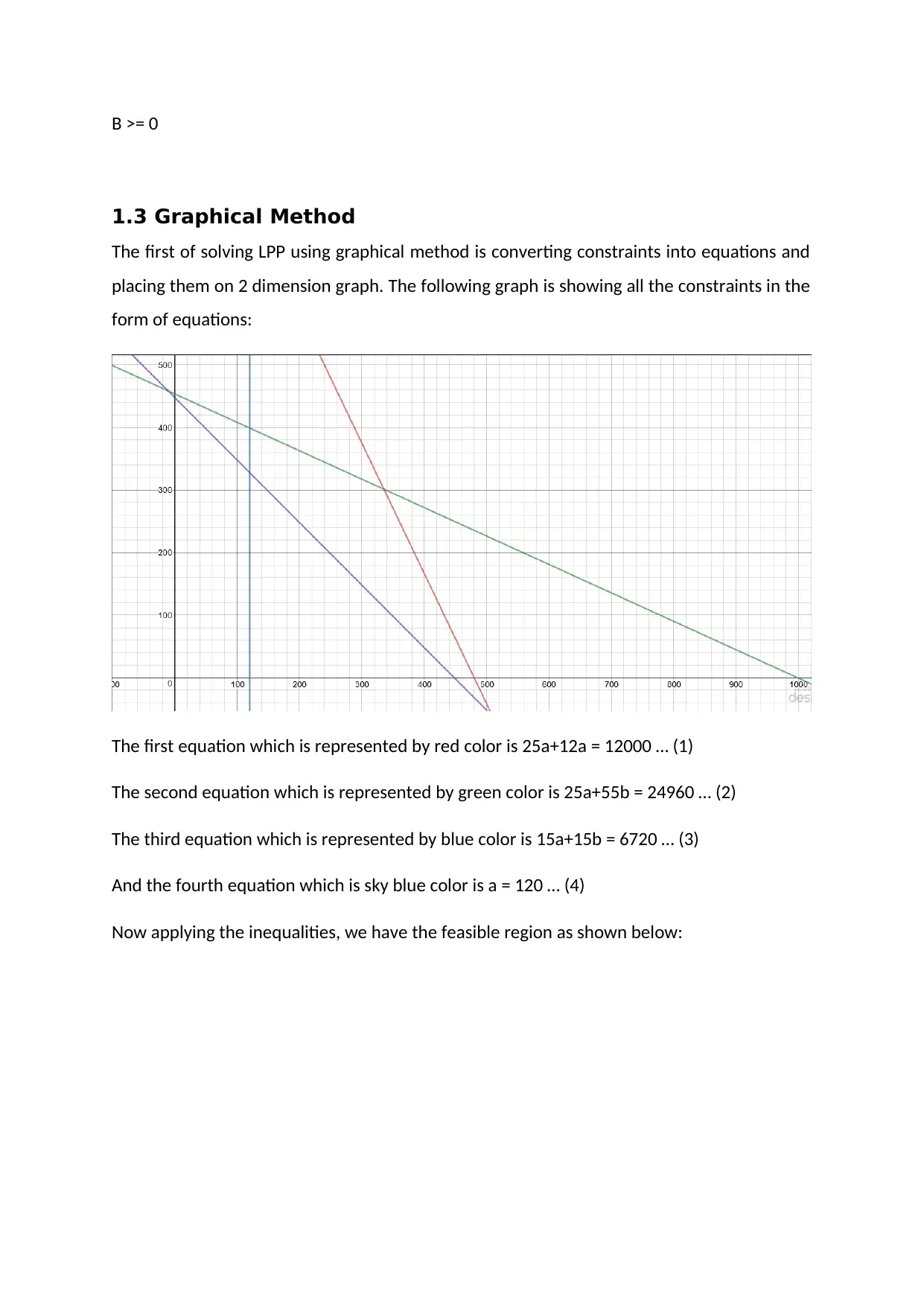
1.3 Graphical Method
The first of solving LPP using graphical method is converting constraints into equations and
placing them on 2 dimension graph. The following graph is showing all the constraints in the
form of equations:
The first equation which is represented by red color is 25a+12a = 12000 … (1)
The second equation which is represented by green color is 25a+55b = 24960 … (2)
The third equation which is represented by blue color is 15a+15b = 6720 … (3)
And the fourth equation which is sky blue color is a = 120 … (4)
Now applying the inequalities, we have the feasible region as shown below:

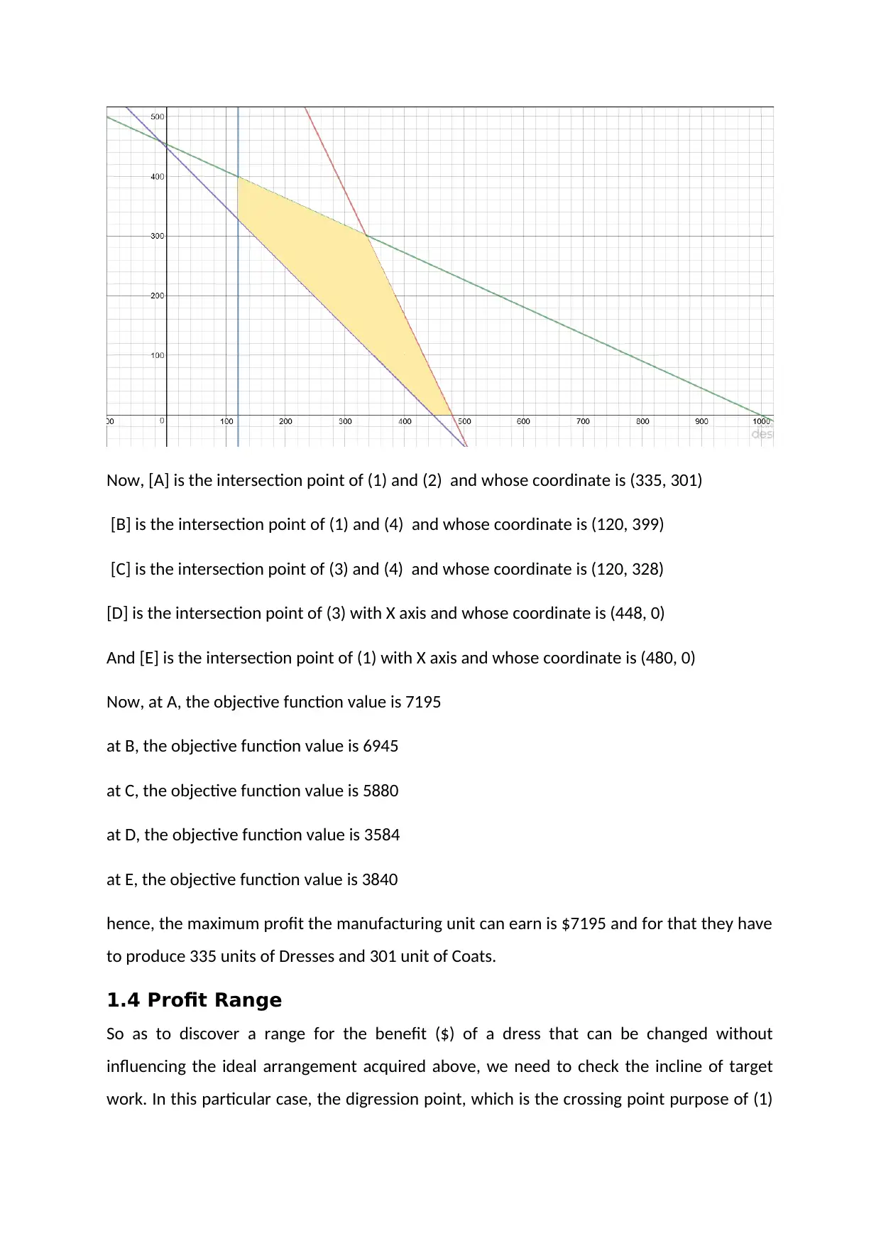
Now, [A] is the intersection point of (1) and (2) and whose coordinate is (335, 301)
[B] is the intersection point of (1) and (4) and whose coordinate is (120, 399)
[C] is the intersection point of (3) and (4) and whose coordinate is (120, 328)
[D] is the intersection point of (3) with X axis and whose coordinate is (448, 0)
And [E] is the intersection point of (1) with X axis and whose coordinate is (480, 0)
Now, at A, the objective function value is 7195
at B, the objective function value is 6945
at C, the objective function value is 5880
at D, the objective function value is 3584
at E, the objective function value is 3840
hence, the maximum profit the manufacturing unit can earn is $7195 and for that they have
to produce 335 units of Dresses and 301 unit of Coats.
1.4 Profit Range
So as to discover a range for the benefit ($) of a dress that can be changed without
influencing the ideal arrangement acquired above, we need to check the incline of target
work. In this particular case, the digression point, which is the crossing point purpose of (1)

and (2) achieved greatest benefit. Consequently, it very well may be said that there is just a
single point and henceforth, rather than range, the X esteem will be 335 as it were.
Answer to question 2
2.1 LPP formulation
Let A denotes number of boxes of cereals A, B denotes number of boxes of cereals B and C
denotes number of boxes of cereals C to be manufactured.
Now, the total revenue from these three types of cereals can be calculated as:
2.60*A + 2.30*B + 3.20*C
On the other hand, the production cost of each box of cereals can be calculated as:
(4.20/500)*A + (2.60/500)*B + (3.00/500)*C
At the same time, the total raw material costs of each type of box can be calculated as:
(100/500)*(0.80A + 0.60B + 0.45C) + (90/500)*(0.10A + 0.25B + 0.15C) + (110/500)*(0.05A +
0.05B + 0.10C) + (200/500)*(0.05A + 0.10B + 0.30C)
Hence, the total cost is:
(4.20/500)A + (2.60/500)B + (3.00/500)C + (100/500)*(0.80A + 0.60B + 0.45A) +
(90/500)*(0.10A + 0.25B + 0.15C) + (110/500)*(0.05A + 0.05B + 0.10C) + (200/500)*(0.05A +
0.10B + 0.30C)
= 0.2075A + 0.2212B + 0.2650C
Therefore, the total profit will be:
2.60A + 2.30B + 3.20C – (0.2075A + 0.2212B + 0.2650C)
=2.3925A + 2.0788B + 2.935C
Therefore, the objective function will be
Max 2.3925A + 2.0788B + 2.935C
Now the constraints are given as
A >= 1000

B >= 800
C >= 750
And
0.80A + 0.60B + 0.45C <= 10000
0.10A + 0.25B + 0.15C <= 5000
0.05A + 0.05B + 0.10C <= 2000
0.05A + 0.10B + 0.30C <= 2000
2.2 R code
install.packages("lpSolve")
require(lpSolve)
X <- c(2.3925, 2.0788, 2.935)
Y <- matrix(c(1, 0, 0,
0, 1, 0,
0, 0, 1,
0.80, 0.60, 0.45,
0.10, 0.25, 0.15,
0.05, 0.05, 0.10,
0.05, 0.10, 0.30), nrow=7, byrow=TRUE)
Z <- c(1000, 800, 750, 10000, 5000, 2000, 2000)
Constranints <- c(">=", ">=", ">=", "<=", "<=", "<=", "<=")
Calculations <- lp(direction="max",
objective.in = X,
const.mat = Y,
const.dir = Constranints,
const.rhs = Z,
all.int = T)
print(Calculations$status)
Solution <- optimum$solution
names(Solution) <- c("Cereal A", "Cereal B", "Cereal C")
print(Solution)
print(paste("Optimum Profit= $", round(Calculations$objval,digits=2), sep=""))
Optimal solution:

Answer to question 3
3.1 Two players zero sum game
A two-player game is known as a zero sum game if the entirety of the two result matrices is
zero. The result to one player is constantly made by the other player (no externalities). For
this situation as the total of two result frameworks is zero, we can say that this game is a
two person zero sum game.
3.2 Payoff Matrix
(Alice, John) John
(4,0) (3,1) (2,2) (1,3) (0,4)
Alice
(5,0) (1,-1) (0,0) (0,0) (0,0) (1,-1)
(4,1) (1,-1) (1,-1) (0,0) (1,-1) (1,-1)
(3,2) (0,0) (1,-1) (2,-2) (1,-1) (0,0)
(2,3) (0,0) (1,-1) (2,-2) (1,-1) (1,-1)
(1,4) (1,-1) (1,-1) (0,0) (1,-1) (1,-1)
(0,5) (1,-1) (0,0) (0,0) (0,0) (1,-1)
3.3 Saddle Point
Saddle point in game theory refers to a value of a function of two player which is a
maximum with respect to one and a minimum with respect to the other.
This game does not have any saddle point.
3.4 Formulation of LPP
For, Alice the linear programming model will look like:
Min 1/V = a1 + a2 + a3 + a4 + a5 +a6
Subject to,
1a1 + 1a2 + 0a3 + 0a4 + 1a5 + 1a6 >= 1
0a1 + 1a2 + 1a3 + 1a4 + 1a5 + 0a6 >= 1
0a1 + 0a2 + 2a3 + 2a4 + 0a5 + 0a6 >= 1

0a1 + 1a2 + 1a3 + 1a4 + 1a5 + 0a6 >= 1
1a1 + 1a2 + 0a3 + 1a4 + 1a5 + 1a6 >= 1
a1, a2, a3, a4, a5, a6 >= 0
for John the linear programming model will look like:
Max 1/V = p1 +p2 +p3 +p4 +p5
Subject to,
-1p1 + 0p2 + 0p3 + 0p4 -1p5 <= 1
-1p1 - 1p2 + 0p3 - 1p4 - 1p5 <= 1
0p1 - 1p2 - 2p3 - 1p4 + 0p5 <= 1
0p1 – 1p2 – 2p3 -1p4 – 1p5 <= 1
-1p1 - 1p2 + 0p3 – 1p4 – 1p5 <= 1
-1p1 + 0p2 + 0p3 + 0p4 – 1p5 <= 1
p1, p2, p3, p4, p5 >= 0
3.5 R code
R code:
# For Alice
require(lpSolve)
X <- c(1,1,1,1,1,1)
Y <- matrix(c(1, 1, 0, 0, 1, 1,
0, 1, 1, 1, 1, 0,
0, 0, 2, 2, 0, 0,
0, 1, 1, 1, 1, 0,
1, 1, 0, 1, 1, 1), nrow=5, byrow=TRUE)
Z <- c(1, 1, 1, 1, 1)
Constranints <- c(">=", ">=", ">=", ">=", ">=")
Solutions <- lp(direction="min",
objective.in = X,
const.mat = Y,
const.dir = Constranints,
const.rhs = Z,
all.int = T)
print(Solutions$status)

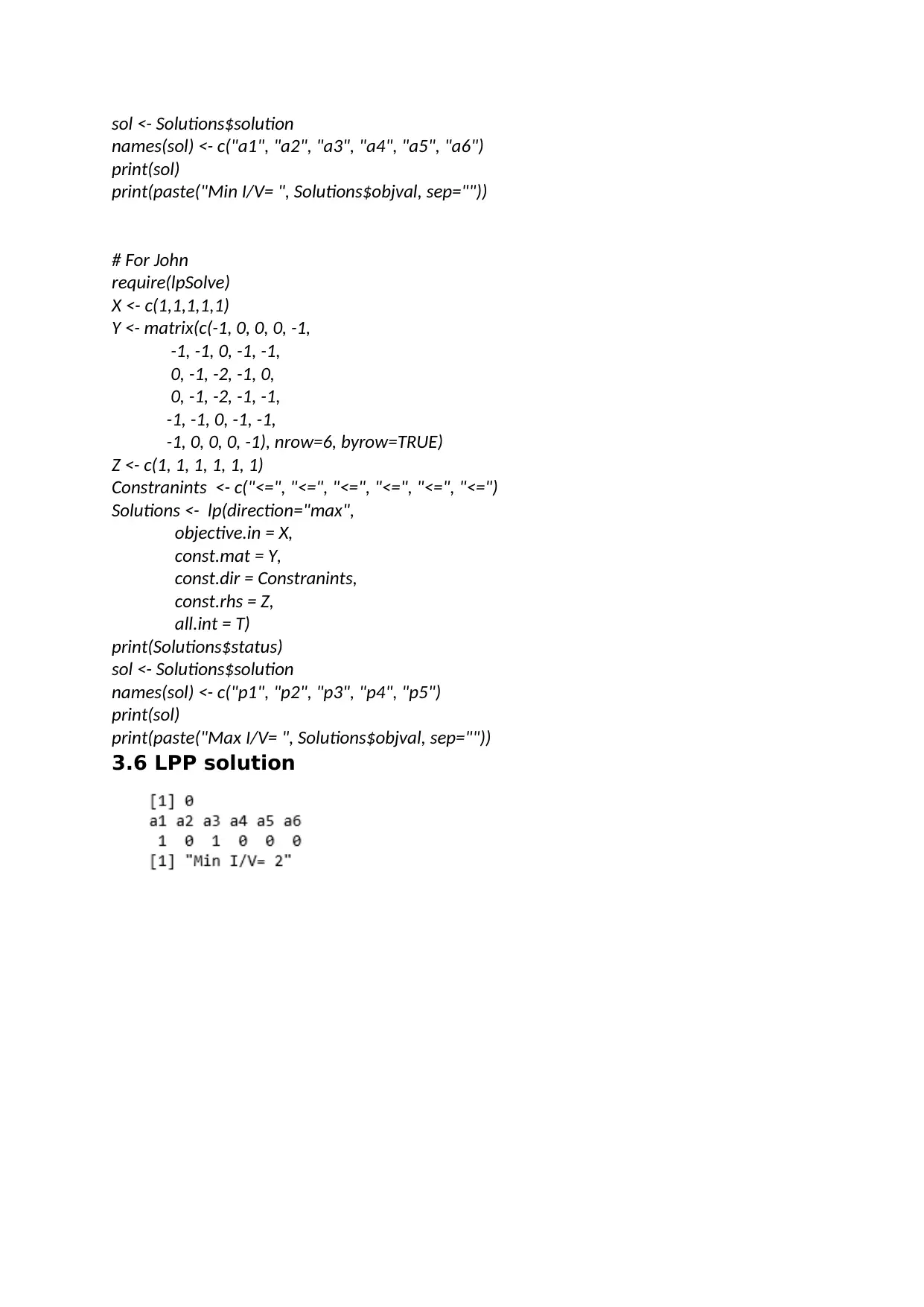
sol <- Solutions$solution
names(sol) <- c("a1", "a2", "a3", "a4", "a5", "a6")
print(sol)
print(paste("Min I/V= ", Solutions$objval, sep=""))
# For John
require(lpSolve)
X <- c(1,1,1,1,1)
Y <- matrix(c(-1, 0, 0, 0, -1,
-1, -1, 0, -1, -1,
0, -1, -2, -1, 0,
0, -1, -2, -1, -1,
-1, -1, 0, -1, -1,
-1, 0, 0, 0, -1), nrow=6, byrow=TRUE)
Z <- c(1, 1, 1, 1, 1, 1)
Constranints <- c("<=", "<=", "<=", "<=", "<=", "<=")
Solutions <- lp(direction="max",
objective.in = X,
const.mat = Y,
const.dir = Constranints,
const.rhs = Z,
all.int = T)
print(Solutions$status)
sol <- Solutions$solution
names(sol) <- c("p1", "p2", "p3", "p4", "p5")
print(sol)
print(paste("Max I/V= ", Solutions$objval, sep=""))
3.6 LPP solution

Reference
Ficken, F.A., 2015. The simplex method of linear programming. Courier Dover Publications.
Korte, B. and Vygen, J., 2018. Linear Programming Algorithms. In Combinatorial
Optimization (pp. 75-102). Springer, Berlin, Heidelberg.
Vanderbei, R.J., 2015. Linear programming. Heidelberg: Springer.