SIT718 Real World Analytics Assignment 1: Linear Programming Solutions
VerifiedAdded on 2022/10/03
|9
|1996
|46
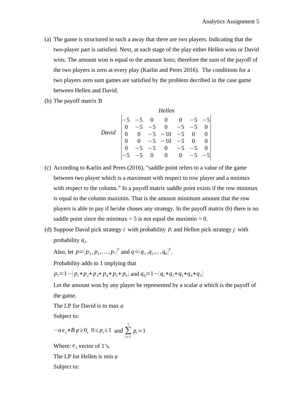
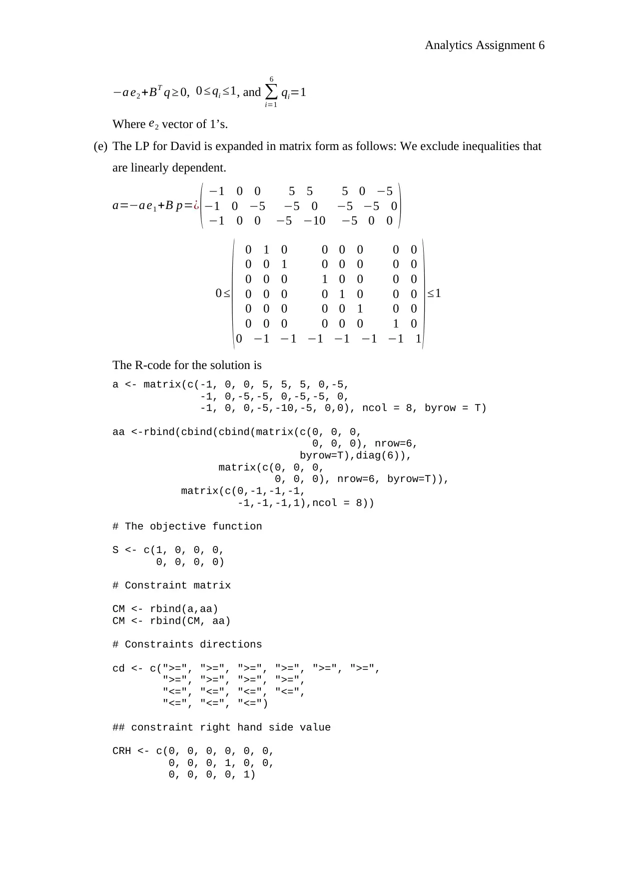
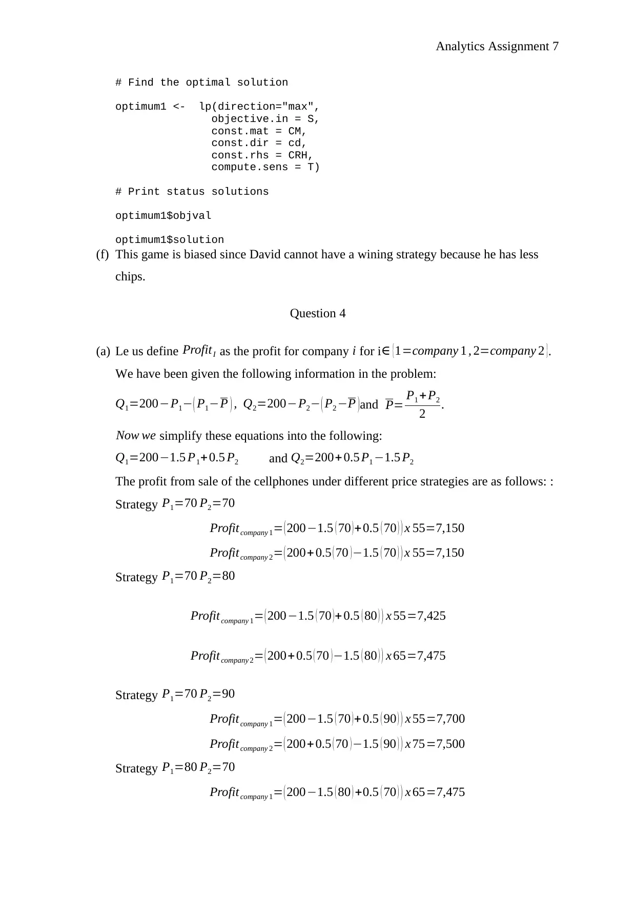
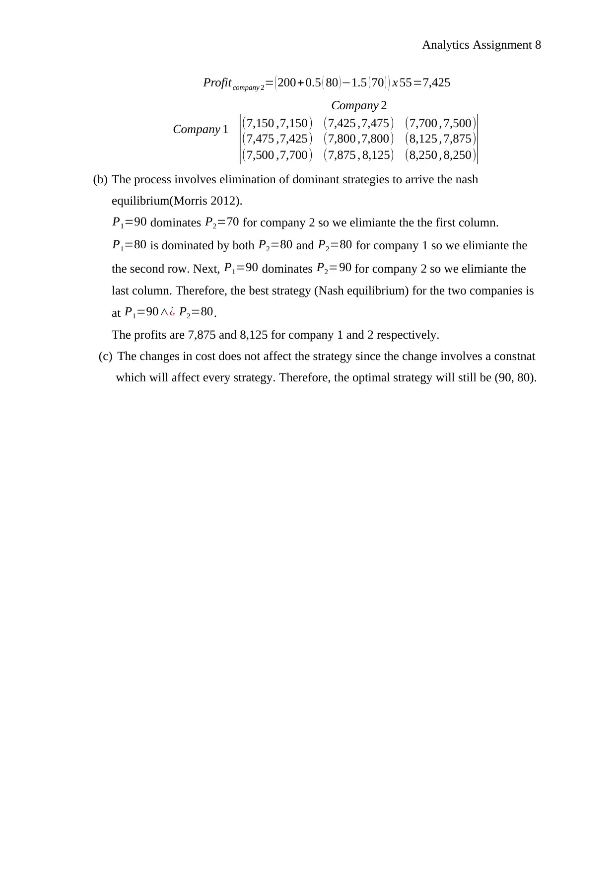
Homework Assignment
AI Summary
This assignment solution covers various problems in real-world analytics. It includes formulating and solving a linear programming problem to minimize costs in a food factory, determining the optimal mix of ingredients for beverage production using Desmos. It also involves solving a product mix problem using R to maximize profit, analyzing a two-player zero-sum game to determine optimal strategies using linear programming, and finding the Nash equilibrium in a pricing game between two companies. The solutions use tools like Desmos and R, and concepts from game theory and linear optimization are applied. Desklib provides access to similar solved assignments and study resources for students.

1 out of 9
Related Documents


![Course Name: Real World Analytics Assignment Solution - [Date]](/_next/image/?url=https%3A%2F%2Fdesklib.com%2Fmedia%2Fimages%2Fjs%2F7cd677b2bca5453d86bfbb121190a9b2.jpg&w=256&q=75)


Your All-in-One AI-Powered Toolkit for Academic Success.
+13062052269
info@desklib.com
Available 24*7 on WhatsApp / Email
![[object Object]](/_next/static/media/star-bottom.7253800d.svg)
Copyright © 2020–2026 A2Z Services. All Rights Reserved. Developed and managed by ZUCOL.