Course Name: Real World Analytics Assignment Solution - [Date]

This document presents a comprehensive solution to a Real World Analytics assignment. The solution begins with a linear programming problem focused on cost minimization, including the formulation of an objective function, constraints, and analysis using Desmos to find the optimal solution. The second question involves maximizing profit using linear programming, incorporating demand constraints and R code for optimization. Finally, the assignment delves into game theory, specifically a two-player zero-sum game, with a payoff matrix analysis and R code implementation to determine the optimal strategies and saddle point. The document includes detailed calculations, explanations, and references to support the solutions.

Real World Analytics 1
REAL WORLD ANALYTICS
By Student Name
Course Name
Professor Name
University Name
City, State
Date

Real World Analytics 2
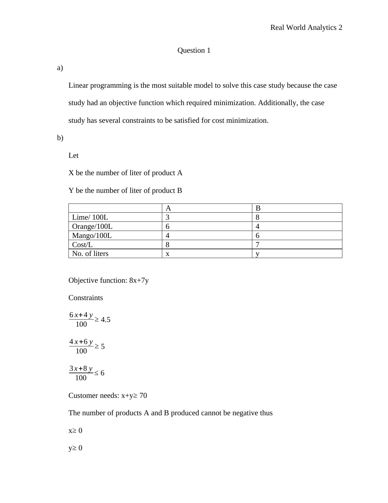
Question 1
a)
Linear programming is the most suitable model to solve this case study because the case
study had an objective function which required minimization. Additionally, the case
study has several constraints to be satisfied for cost minimization.
b)
Let
X be the number of liter of product A
Y be the number of liter of product B
A B
Lime/ 100L 3 8
Orange/100L 6 4
Mango/100L 4 6
Cost/L 8 7
No. of liters x y
Objective function: 8x+7y
Constraints
6 x+ 4 y
100 ≥ 4.5
4 x +6 y
100 ≥ 5
3 x +8 y
100 ≤ 6
Customer needs: x+y≥ 70
The number of products A and B produced cannot be negative thus
x≥ 0
y≥ 0

Real World Analytics 3
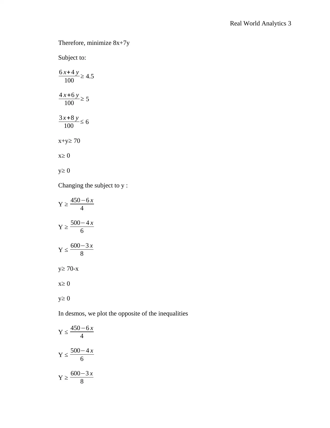
Therefore, minimize 8x+7y
Subject to:
6 x+ 4 y
100 ≥ 4.5
4 x +6 y
100 ≥ 5
3 x +8 y
100 ≤ 6
x+y≥ 70
x≥ 0
y≥ 0
Changing the subject to y :
Y ≥ 450−6 x
4
Y ≥ 500−4 x
6
Y ≤ 600−3 x
8
y≥ 70-x
x≥ 0
y≥ 0
In desmos, we plot the opposite of the inequalities
Y ≤ 450−6 x
4
Y ≤ 500−4 x
6
Y ≥ 600−3 x
8

Real World Analytics 4
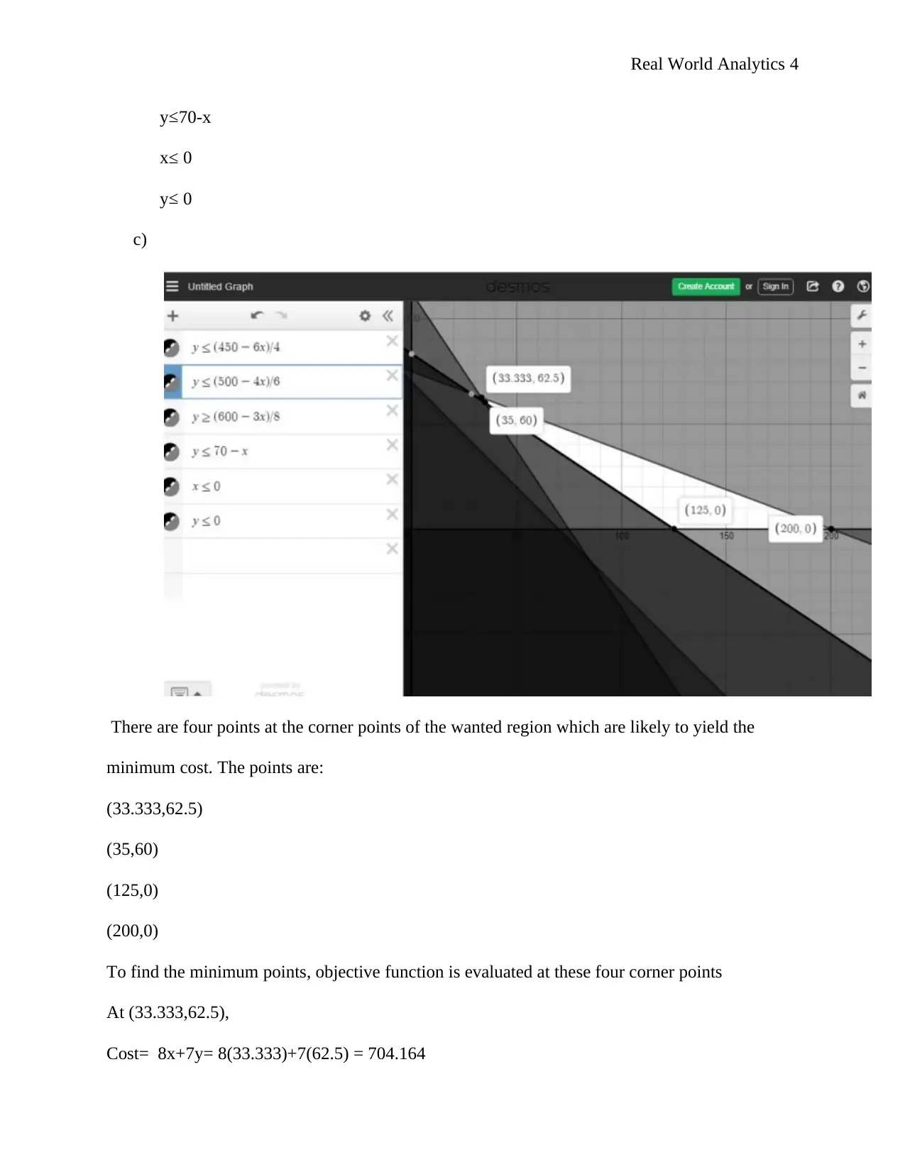
y≤70-x
x≤ 0
y≤ 0
c)
There are four points at the corner points of the wanted region which are likely to yield the
minimum cost. The points are:
(33.333,62.5)
(35,60)
(125,0)
(200,0)
To find the minimum points, objective function is evaluated at these four corner points
At (33.333,62.5),
Cost= 8x+7y= 8(33.333)+7(62.5) = 704.164

Real World Analytics 5
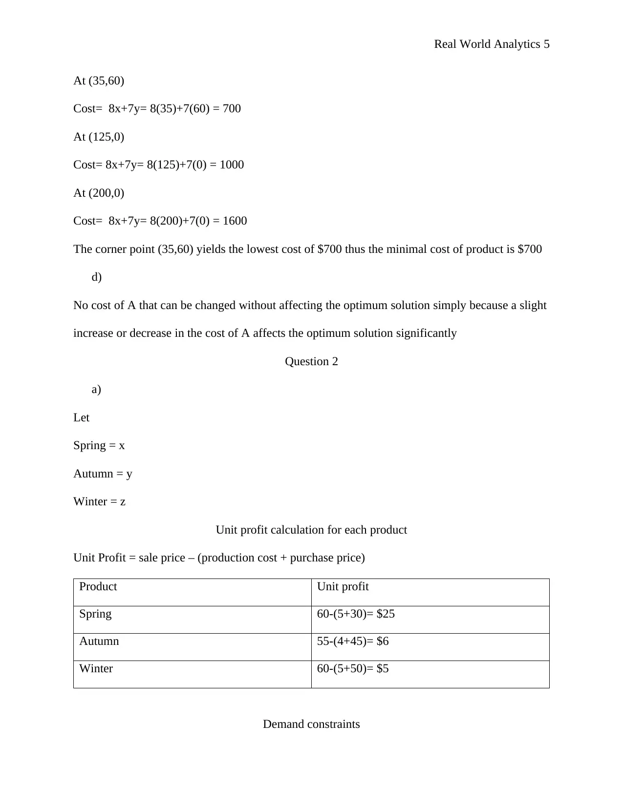
At (35,60)
Cost= 8x+7y= 8(35)+7(60) = 700
At (125,0)
Cost= 8x+7y= 8(125)+7(0) = 1000
At (200,0)
Cost= 8x+7y= 8(200)+7(0) = 1600
The corner point (35,60) yields the lowest cost of $700 thus the minimal cost of product is $700
d)
No cost of A that can be changed without affecting the optimum solution simply because a slight
increase or decrease in the cost of A affects the optimum solution significantly
Question 2
a)
Let
Spring = x
Autumn = y
Winter = z
Unit profit calculation for each product
Unit Profit = sale price – (production cost + purchase price)
Product Unit profit
Spring 60-(5+30)= $25
Autumn 55-(4+45)= $6
Winter 60-(5+50)= $5
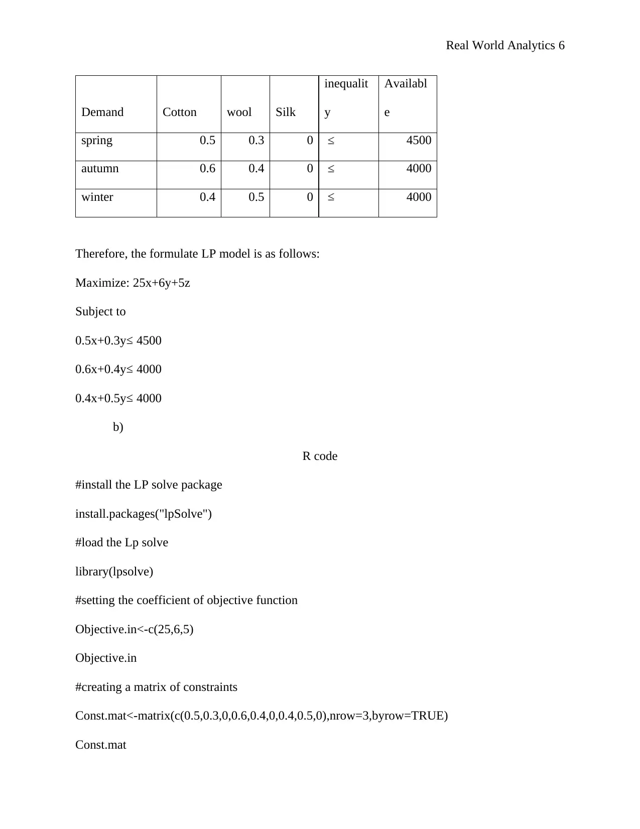
Demand constraints

Real World Analytics 6
Demand Cotton wool Silk
inequalit
y
Availabl
e
spring 0.5 0.3 0 ≤ 4500
autumn 0.6 0.4 0 ≤ 4000
winter 0.4 0.5 0 ≤ 4000
Therefore, the formulate LP model is as follows:
Maximize: 25x+6y+5z
Subject to
0.5x+0.3y ≤ 4500
0.6x+0.4y ≤ 4000
0.4x+0.5y ≤ 4000
b)
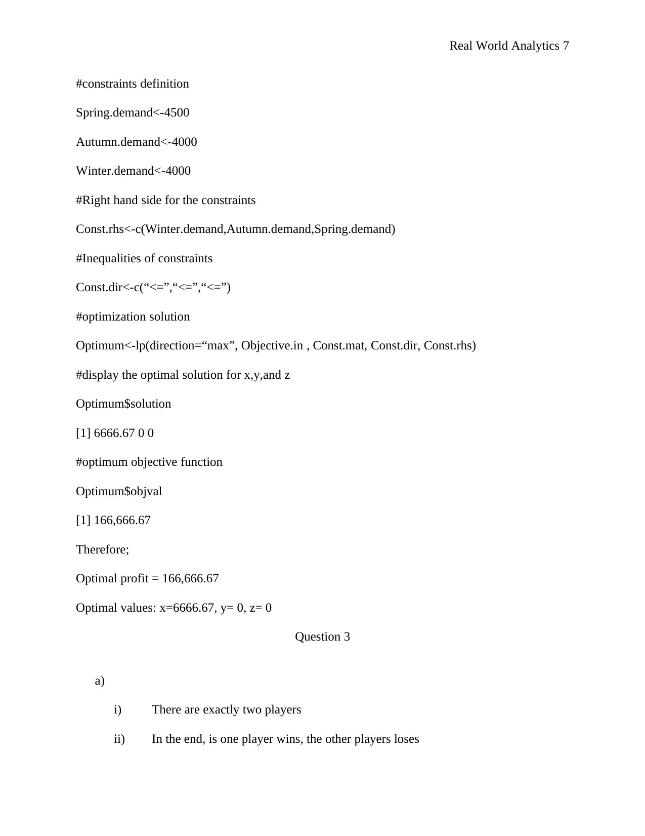
R code
#install the LP solve package
install.packages("lpSolve")
#load the Lp solve
library(lpsolve)
#setting the coefficient of objective function
Objective.in<-c(25,6,5)
Objective.in
#creating a matrix of constraints
Const.mat<-matrix(c(0.5,0.3,0,0.6,0.4,0,0.4,0.5,0),nrow=3,byrow=TRUE)
Const.mat

Real World Analytics 7
#constraints definition
Spring.demand<-4500
Autumn.demand<-4000
Winter.demand<-4000
#Right hand side for the constraints
Const.rhs<-c(Winter.demand,Autumn.demand,Spring.demand)
#Inequalities of constraints
Const.dir<-c(“<=”,“<=”,“<=”)
#optimization solution
Optimum<-lp(direction=“max”, Objective.in , Const.mat, Const.dir, Const.rhs)
#display the optimal solution for x,y,and z
Optimum$solution
[1] 6666.67 0 0
#optimum objective function
Optimum$objval
[1] 166,666.67
Therefore;
Optimal profit = 166,666.67
Optimal values: x=6666.67, y= 0, z= 0
Question 3
a)
i) There are exactly two players
ii) In the end, is one player wins, the other players loses

Real World Analytics 8
iii) One players gain is equivalent to the other players loss
iv) Two-players-zero-sum game is a mathematical representation of one players
utility gain and the other players utility loss in economics whose sum is zero
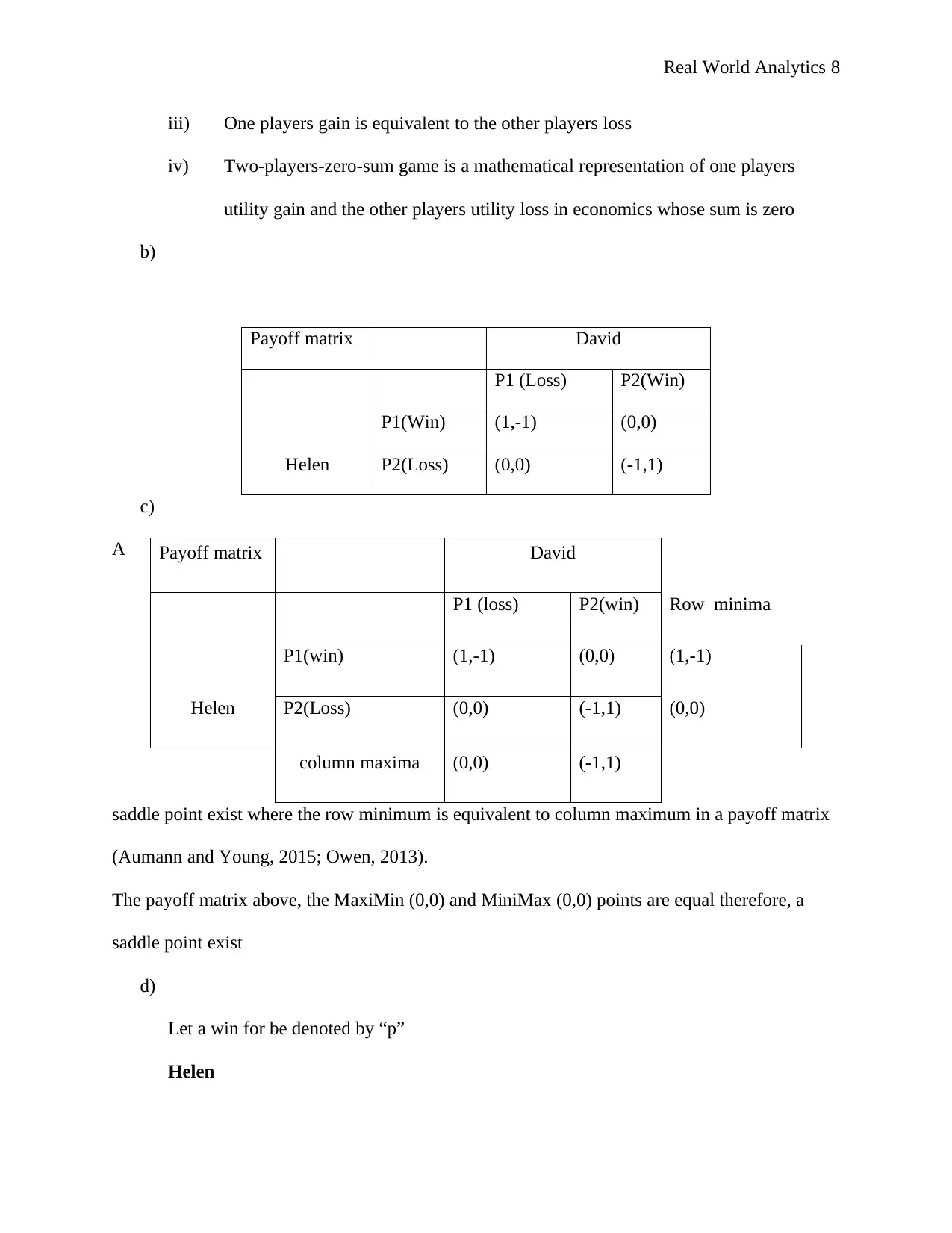
b)
Payoff matrix David
Helen
P1 (Loss) P2(Win)
P1(Win) (1,-1) (0,0)
P2(Loss) (0,0) (-1,1)
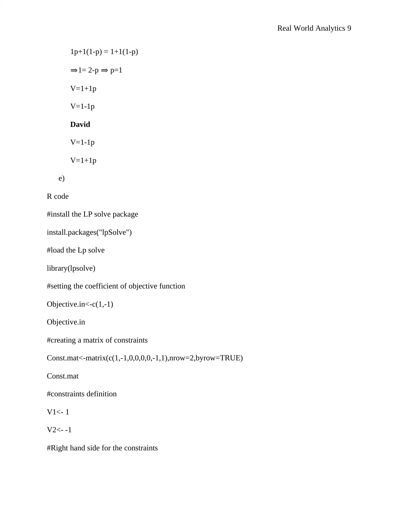
c)
A
saddle point exist where the row minimum is equivalent to column maximum in a payoff matrix
(Aumann and Young, 2015; Owen, 2013).
The payoff matrix above, the MaxiMin (0,0) and MiniMax (0,0) points are equal therefore, a
saddle point exist
d)
Let a win for be denoted by “p”
Helen
Payoff matrix David
Helen
P1 (loss) P2(win) Row minima
P1(win) (1,-1) (0,0) (1,-1)
P2(Loss) (0,0) (-1,1) (0,0)
column maxima (0,0) (-1,1)

Real World Analytics 9
1p+1(1-p) = 1+1(1-p)
⇒1= 2-p ⇒ p=1
V=1+1p
V=1-1p
David
V=1-1p
V=1+1p
e)
R code
#install the LP solve package
install.packages("lpSolve")
#load the Lp solve
library(lpsolve)
#setting the coefficient of objective function
Objective.in<-c(1,-1)
Objective.in
#creating a matrix of constraints
Const.mat<-matrix(c(1,-1,0,0,0,0,-1,1),nrow=2,byrow=TRUE)
Const.mat
#constraints definition
V1<- 1
V2<- -1
#Right hand side for the constraints

Real World Analytics 10
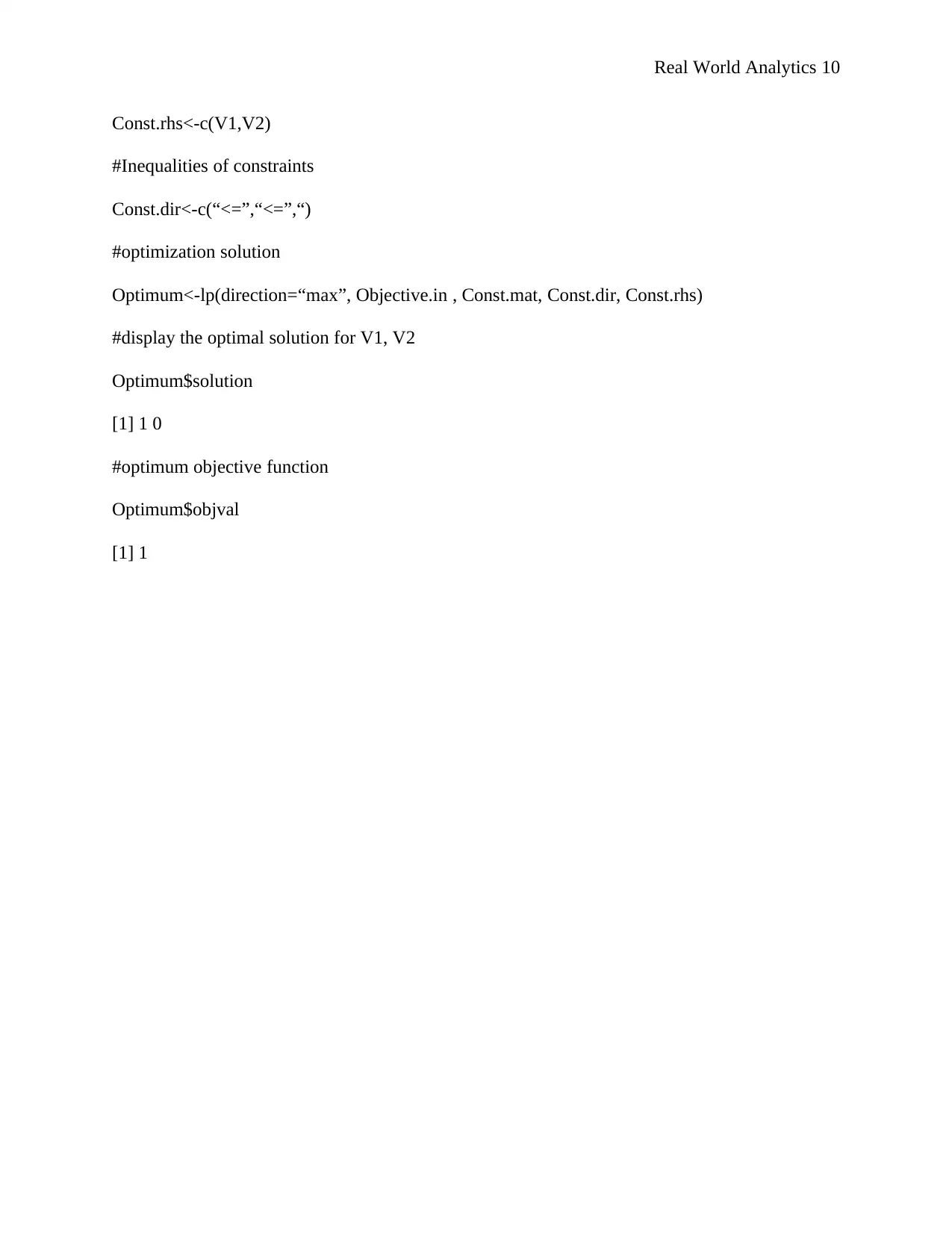
Const.rhs<-c(V1,V2)
#Inequalities of constraints
Const.dir<-c(“<=”,“<=”,“)
#optimization solution
Optimum<-lp(direction=“max”, Objective.in , Const.mat, Const.dir, Const.rhs)
#display the optimal solution for V1, V2
Optimum$solution
[1] 1 0
#optimum objective function
Optimum$objval
[1] 1

Real World Analytics 11
References
Aumann, R. and Young, H. (2015). Handbook of game theory. Amsterdam: North-Holland.
Owen, G. (2013). Applications of game theory to economics. International Game Theory
Review, 15(03), p.1340011.