SIT718 Real World Analytics: Data Analysis and Aggregation Functions

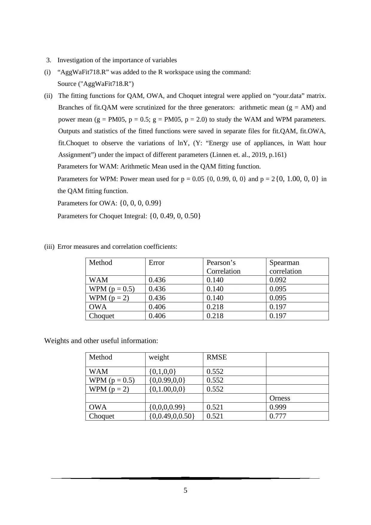
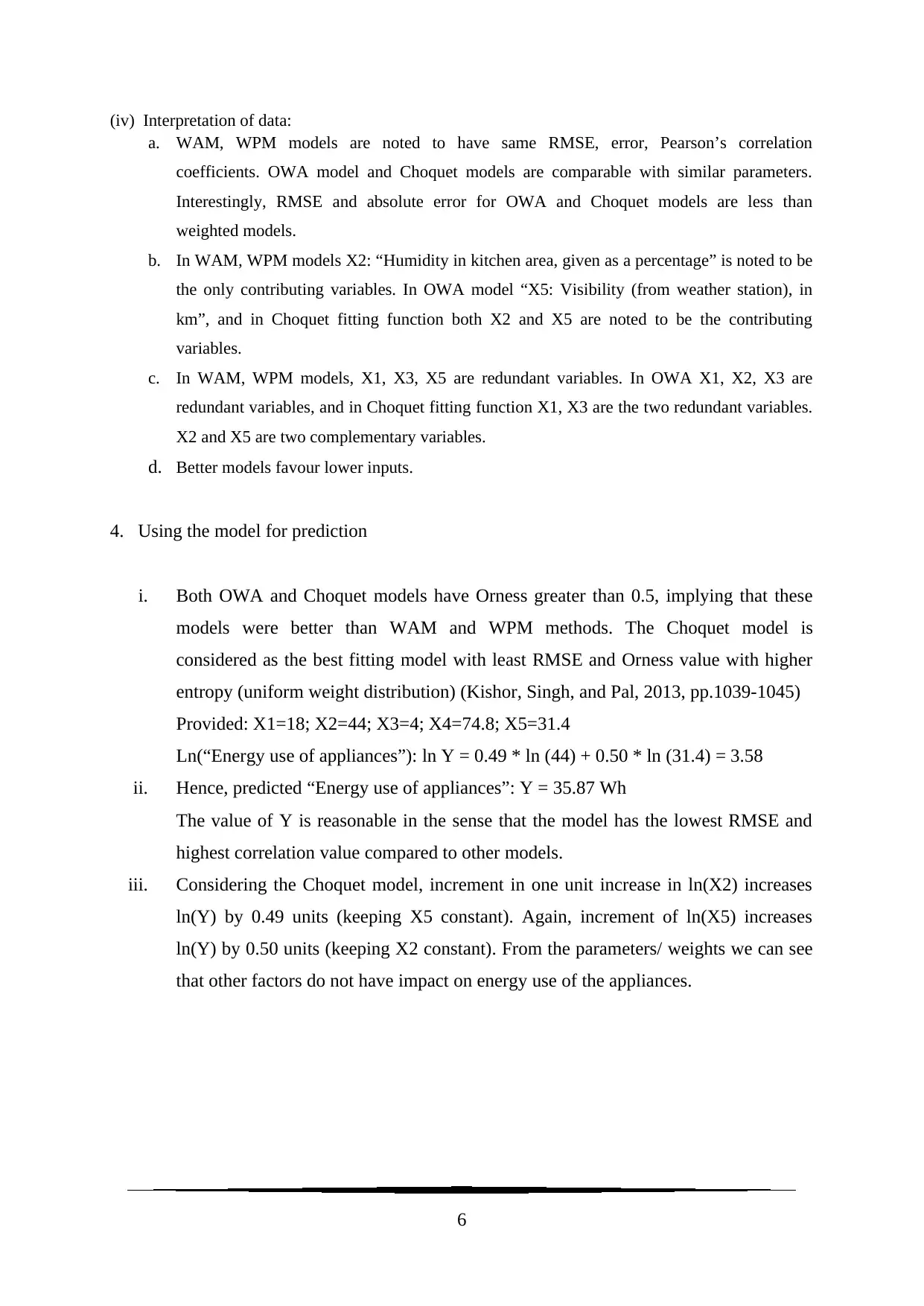
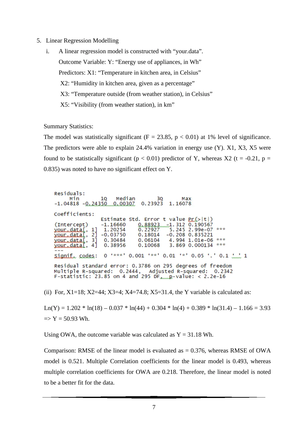
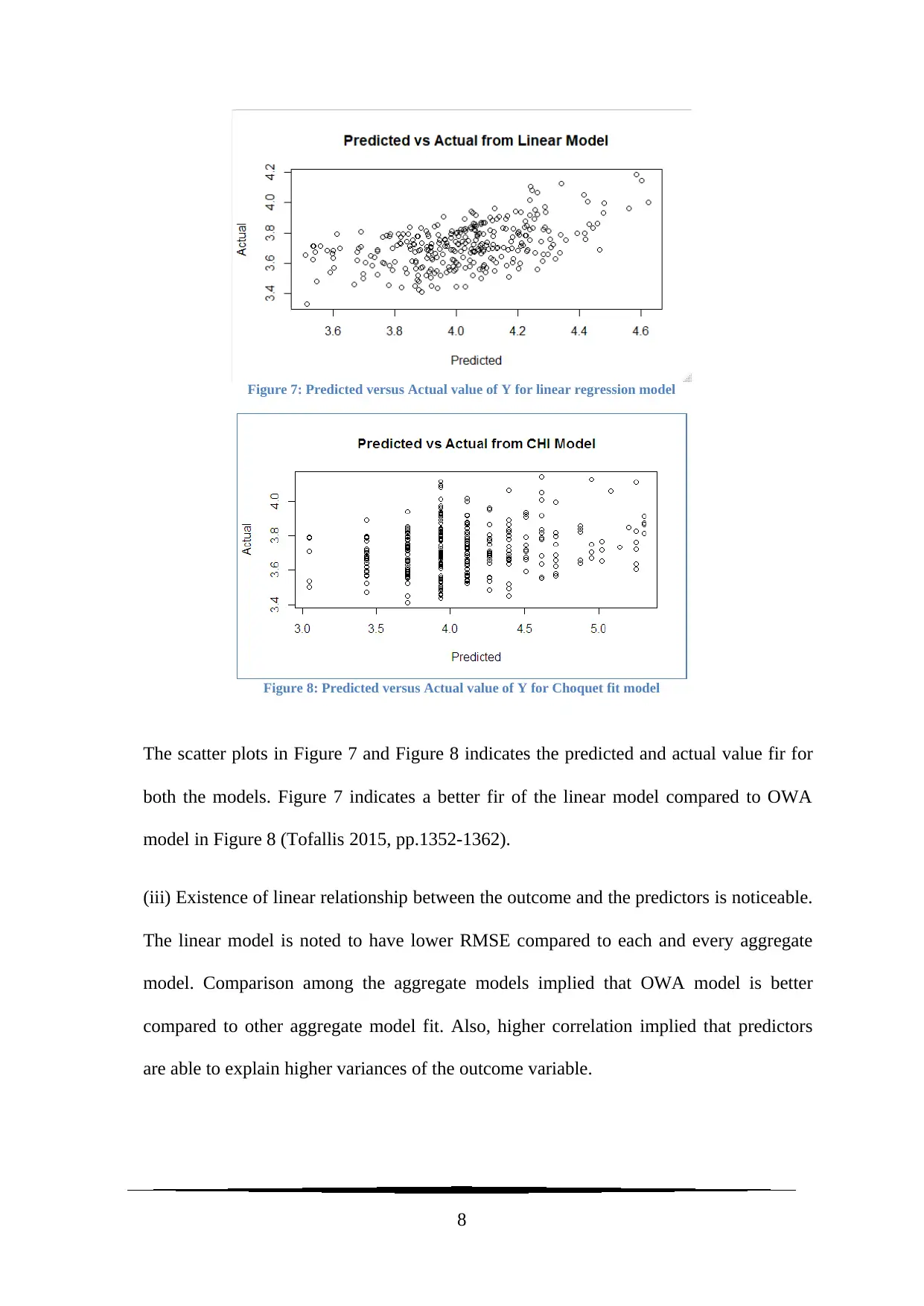
This assignment solution for SIT718 Real World Analytics focuses on data understanding and analysis using R programming. The task involves importing and manipulating a dataset, generating histograms and scatter plots to understand the data distribution and relationships between variables. The solution then explores data transformation techniques, excluding an irrelevant variable and applying logarithmic transformations. The core of the assignment lies in investigating the importance of variables using aggregation functions like QAM, OWA, and Choquet integral, comparing their performance based on error measures and correlation coefficients. Finally, the solution uses the models for prediction and constructs a linear regression model for comparison, evaluating their performance using RMSE and correlation coefficients, and providing interpretations of the results. The findings highlight the effectiveness of different models and the significance of various variables in predicting the outcome variable. The assignment also includes references to relevant research papers to support the analysis.

SIT718 Real World Analytics
1

Assignment Task
1. Data Understanding
(i) “Energy19.txt” downloaded and added to the R working directory.
(ii) Data assigned to matrix using the command:
the.data <- as.matrix(read.table("Energy19.txt "))
(iii) A subset of 300 data generated using the command:
my.data <- the.data[sample(1:671,300),c(1:6)]
(iv) Histograms for all the six variables are as follows:
Figure 1: Histogram for Temperature in kitchen area (Celsius) and Histogram for humidity in kitchen area (%)
Figure 2: Histogram for temperature outside kitchen area and Histogram for outside humidity (%)
2

Figure 3: Histogram for visibility (km) and for energy use of appliances
Figure 4: Scatter plots of energy use of appliances on temperature and humidity in kitchen area
Figure 5: Scatter plot of energy use of appliances on temperature and humidity outside kitchen area
Figure 6: Scatter plot of energy use of appliances on visibility from weather station
3

X1: “Temperature in kitchen area, in Celsius”
From the histogram in Figure 1, this variable is noted to be almost normally distributed. Figure 8
represents a moderately positive correlation with energy uses of appliances.
X2: “Humidity in kitchen area, given as a percentage”
From the histogram in Figure 2, this variable is noted to be almost normally distributed with a
slight right Skewness. Figure 7 represents a low positive correlation with energy uses of
appliances.
X3: “Temperature outside (from weather station), in Celsius”
From the histogram in Figure 3, this variable is noted to be slightly left skewed. Figure 9
represents a moderate positive correlation with energy uses of appliances.
X4: “Humidity outside (from weather station), given as a percentage”
From the histogram in Figure 4, this variable is noted to be almost normal with slightly left
skewed distribution. Figure 10 represents a very low positive correlation with energy uses of
appliances.
X5: “Visibility (from weather station), in km”
From the histogram in Figure 5, this variable is noted to be almost normal with presence of few
higher values as outliers. Figure 11 represents a low positive correlation with energy uses of
appliances.
Y: “Energy use of appliances, in Watt hour Assignment”
From the histogram in Figure 6, this variable is noted to be highly right skewed with unusually
higher data for energy uses (Vartak et. al., 2015, pp.2182-2193)
.
2. Transformation of the data
(i) Considering the correlations and shape of the distributions, X4: “Humidity outside (from weather
station), given as a percentage” was excluded from the list of predictors. Hence, X1, X2, X3, X5,
and Y have been selected. The data was saved in a file named “name-transformed.txt”.
(ii)Logarithmic transformation (natural log) was applied to the outcome and predictor variables. The
log transformation was used to make highly skewed outcome variable Y: “Energy use of
appliances, in Watt hour Assignment” less skewed. This was valuable for making patterns in the
outcome variable more interpretable satisfying the assumptions of inferential statistics (Khademi
et. al., 2016, pp.355-369)
4

3. Investigation of the importance of variables
(i) “AggWaFit718.R” was added to the R workspace using the command:
Source ("AggWaFit718.R")
(ii) The fitting functions for QAM, OWA, and Choquet integral were applied on “your.data” matrix.
Branches of fit.QAM were scrutinized for the three generators: arithmetic mean (g = AM) and
power mean (g = PM05, p = 0.5; g = PM05, p = 2.0) to study the WAM and WPM parameters.
Outputs and statistics of the fitted functions were saved in separate files for fit.QAM, fit.OWA,
fit.Choquet to observe the variations of lnY, (Y: “Energy use of appliances, in Watt hour
Assignment”) under the impact of different parameters (Linnen et. al., 2019, p.161)
Parameters for WAM: Arithmetic Mean used in the QAM fitting function.
Parameters for WPM: Power mean used for p = 0.05 {0, 0.99, 0, 0} and p = 2{0, 1.00, 0, 0} in
the QAM fitting function.
Parameters for OWA: {0, 0, 0, 0.99}
Parameters for Choquet Integral: {0, 0.49, 0, 0.50}
(iii) Error measures and correlation coefficients:
Method Error Pearson’s
Correlation
Spearman
correlation
WAM 0.436 0.140 0.092
WPM (p = 0.5) 0.436 0.140 0.095
WPM (p = 2) 0.436 0.140 0.095
OWA 0.406 0.218 0.197
Choquet 0.406 0.218 0.197
Weights and other useful information:
Method weight RMSE
WAM {0,1,0,0} 0.552
WPM (p = 0.5) {0,0.99,0,0} 0.552
WPM (p = 2) {0,1.00,0,0} 0.552
Orness
OWA {0,0,0,0.99} 0.521 0.999
Choquet {0,0.49,0,0.50} 0.521 0.777
5

(iv) Interpretation of data:
a. WAM, WPM models are noted to have same RMSE, error, Pearson’s correlation
coefficients. OWA model and Choquet models are comparable with similar parameters.
Interestingly, RMSE and absolute error for OWA and Choquet models are less than
weighted models.
b. In WAM, WPM models X2: “Humidity in kitchen area, given as a percentage” is noted to be
the only contributing variables. In OWA model “X5: Visibility (from weather station), in
km”, and in Choquet fitting function both X2 and X5 are noted to be the contributing
variables.
c. In WAM, WPM models, X1, X3, X5 are redundant variables. In OWA X1, X2, X3 are
redundant variables, and in Choquet fitting function X1, X3 are the two redundant variables.
X2 and X5 are two complementary variables.
d. Better models favour lower inputs.
4. Using the model for prediction
i. Both OWA and Choquet models have Orness greater than 0.5, implying that these
models were better than WAM and WPM methods. The Choquet model is
considered as the best fitting model with least RMSE and Orness value with higher
entropy (uniform weight distribution) (Kishor, Singh, and Pal, 2013, pp.1039-1045)
Provided: X1=18; X2=44; X3=4; X4=74.8; X5=31.4
Ln(“Energy use of appliances”): ln Y = 0.49 * ln (44) + 0.50 * ln (31.4) = 3.58
ii. Hence, predicted “Energy use of appliances”: Y = 35.87 Wh
The value of Y is reasonable in the sense that the model has the lowest RMSE and
highest correlation value compared to other models.
iii. Considering the Choquet model, increment in one unit increase in ln(X2) increases
ln(Y) by 0.49 units (keeping X5 constant). Again, increment of ln(X5) increases
ln(Y) by 0.50 units (keeping X2 constant). From the parameters/ weights we can see
that other factors do not have impact on energy use of the appliances.
6

5. Linear Regression Modelling
i. A linear regression model is constructed with “your.data”.
Outcome Variable: Y: “Energy use of appliances, in Wh”
Predictors: X1: “Temperature in kitchen area, in Celsius”
X2: “Humidity in kitchen area, given as a percentage”
X3: “Temperature outside (from weather station), in Celsius”
X5: “Visibility (from weather station), in km”
Summary Statistics:
The model was statistically significant (F = 23.85, p < 0.01) at 1% level of significance.
The predictors were able to explain 24.4% variation in energy use (Y). X1, X3, X5 were
found to be statistically significant (p < 0.01) predictor of Y, whereas X2 (t = -0.21, p =
0.835) was noted to have no significant effect on Y.
(ii) For, X1=18; X2=44; X3=4; X4=74.8; X5=31.4, the Y variable is calculated as:
Ln(Y) = 1.202 * ln(18) – 0.037 * ln(44) + 0.304 * ln(4) + 0.389 * ln(31.4) – 1.166 = 3.93
=> Y = 50.93 Wh.
Using OWA, the outcome variable was calculated as Y = 31.18 Wh.
Comparison: RMSE of the linear model is evaluated as = 0.376, whereas RMSE of OWA
model is 0.521. Multiple Correlation coefficients for the linear model is 0.493, whereas
multiple correlation coefficients for OWA are 0.218. Therefore, the linear model is noted
to be a better fit for the data.
7

Figure 7: Predicted versus Actual value of Y for linear regression model
Figure 8: Predicted versus Actual value of Y for Choquet fit model
The scatter plots in Figure 7 and Figure 8 indicates the predicted and actual value fir for
both the models. Figure 7 indicates a better fir of the linear model compared to OWA
model in Figure 8 (Tofallis 2015, pp.1352-1362).
(iii) Existence of linear relationship between the outcome and the predictors is noticeable.
The linear model is noted to have lower RMSE compared to each and every aggregate
model. Comparison among the aggregate models implied that OWA model is better
compared to other aggregate model fit. Also, higher correlation implied that predictors
are able to explain higher variances of the outcome variable.
8

References
Khademi, F., Jamal, S.M., Deshpande, N. and Londhe, S., 2016. Predicting strength of
recycled aggregate concrete using artificial neural network, adaptive neuro-fuzzy inference
system and multiple linear regression. International Journal of Sustainable Built
Environment, 5(2), pp.355-369.
Kishor, A., Singh, A.K. and Pal, N.R., 2013. Orness measure of OWA operators: a new
approach. IEEE Transactions on Fuzzy Systems, 22(4), pp.1039-1045.
Linnen, D.T., Escobar, G.J., Hu, X., Scruth, E., Liu, V. and Stephens, C., 2019. Statistical
modeling and aggregate-weighted scoring systems in prediction of mortality and ICU
transfer: a systematic review. Journal of hospital medicine, 14(3), p.161.
Tofallis, C., 2015. A better measure of relative prediction accuracy for model selection and
model estimation. Journal of the Operational Research Society, 66(8), pp.1352-1362.
Vartak, M., Rahman, S., Madden, S., Parameswaran, A. and Polyzotis, N., 2015. S ee DB:
efficient data-driven visualization recommendations to support visual analytics. Proceedings
of the VLDB Endowment, 8(13), pp.2182-2193.
9