Computational Problem Solving: Lecture Notes on Recurrence Relations
VerifiedAdded on 2023/01/13
|20
|6833
|97
Homework Assignment
AI Summary
This document comprises lecture notes from a Computational Problem Solving course, focusing on recurrence relations and recursive algorithms. It begins with an introduction to recursive algorithms, using the factorial function as an example, and then delves into the classic Towers of Hanoi problem, detailing the problem's constraints, solution strategy, and the derivation of the minimum number of moves (2^n - 1) through mathematical induction. The notes then formally define recurrence relations, distinguishing between linear homogeneous and non-homogeneous types. The Fibonacci and Lucas sequences are used as applications, and the document concludes with an overview of recursion implementation in Python, accompanied by example code. This assignment is available on Desklib, providing students with comprehensive study resources.
Lecture Notes
Computational Problem Solving
Week 7:
Recurrence Relations and Algorithms
Contents
Recursive Algorithms ............................................................................................................................................. 1
Towers of Hanoi .................................................................................................................................................... 1
Recurrence Relations ............................................................................................................................................ 5
Second Order Linear Homogeneous Recurrence Relations .................................................................................. 8
Application: Fibonacci and Lucas Recurrence Relations ....................................................................................... 9
Extension Topic: General Homogeneous Recurrence Relations ......................................................................... 11
Extension Topic: Non-homogeneous Recurrence Relations ........................................................................... 12
Recursion in Python ............................................................................................................................................ 13
Recursive Algorithms
Recursive algorithms are those that call themselves. For example, to find the factorial of an integer is:
5! = 5 × 4 × 3 × 2 × 1
And more generally as:
𝑛! = 𝑛 ×(𝑛 − 1) × (𝑛 − 2) × … × 3 × 2 × 1
As (𝑛 − 1)! =(𝑛 − 1) × (𝑛 − 2) × … × 3 × 2 × 1we can rewrite the above as:
𝑛! = 𝑛 ×(𝑛 − 1)!
Where 1! = 1as a base condition. As we can see recursive algorithms have similar ideas to what we used to
prove statements by mathematical induction.
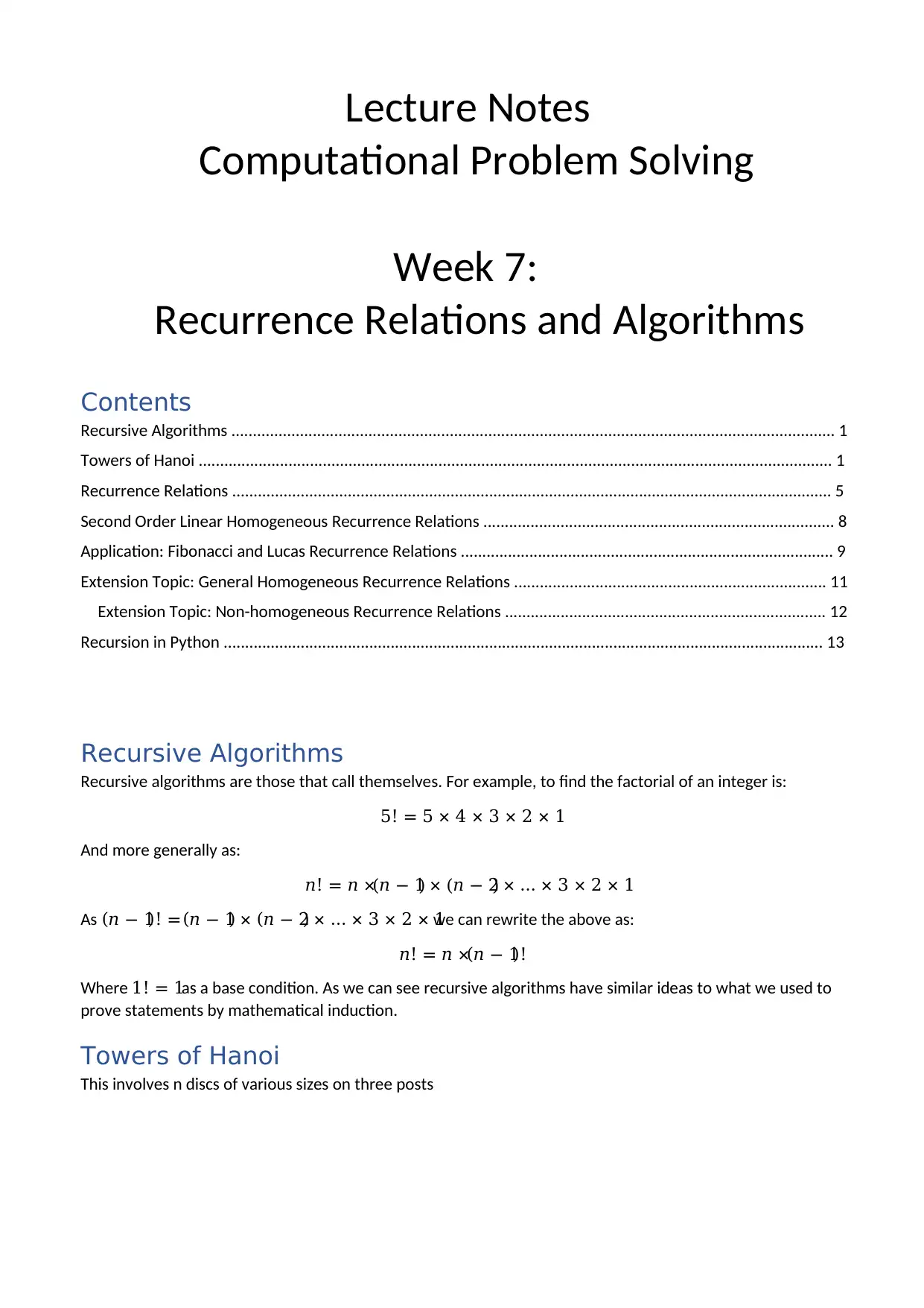
Towers of Hanoi
This involves n discs of various sizes on three posts
Computational Problem Solving
Week 7:
Recurrence Relations and Algorithms
Contents
Recursive Algorithms ............................................................................................................................................. 1
Towers of Hanoi .................................................................................................................................................... 1
Recurrence Relations ............................................................................................................................................ 5
Second Order Linear Homogeneous Recurrence Relations .................................................................................. 8
Application: Fibonacci and Lucas Recurrence Relations ....................................................................................... 9
Extension Topic: General Homogeneous Recurrence Relations ......................................................................... 11
Extension Topic: Non-homogeneous Recurrence Relations ........................................................................... 12
Recursion in Python ............................................................................................................................................ 13
Recursive Algorithms
Recursive algorithms are those that call themselves. For example, to find the factorial of an integer is:
5! = 5 × 4 × 3 × 2 × 1
And more generally as:
𝑛! = 𝑛 ×(𝑛 − 1) × (𝑛 − 2) × … × 3 × 2 × 1
As (𝑛 − 1)! =(𝑛 − 1) × (𝑛 − 2) × … × 3 × 2 × 1we can rewrite the above as:
𝑛! = 𝑛 ×(𝑛 − 1)!
Where 1! = 1as a base condition. As we can see recursive algorithms have similar ideas to what we used to
prove statements by mathematical induction.
Towers of Hanoi
This involves n discs of various sizes on three posts
Paraphrase This Document
Need a fresh take? Get an instant paraphrase of this document with our AI Paraphraser

The disc starts on one of the posts with the largest disc on the bottom of the stack, with the smaller discs
resting on top of a larger disc, so ordered with respect to size.
The exercise is to move all the discs to another post, with the largest on the bottom and the smallest on top
without a larger disc resting on a small disc.
The question is: what is the minimum number of moves needed?
Understanding the Problem:
Objective:
Place the pile of discs on a different peg
Constraints:
- no disc can sit on a smaller disc
- only top disc may be moved
- you can only move one disc at a time
We are being asked to work out the minimum number of moves to move the discs from one peg to another.
We could build a model of the problem (as it was originally in Vietnam). Or we can use diagrams to help us
model the moves. We cannot really restate the problem.
The unknown is the minimum number of moves as well as the number of discs. Also, we are not sure how we
can make those moves to obtain the minimal number of moves. We have not made any assumptions apart
from the constraints of the problem and that there are a fixed number of pegs which is 3 (i.e. we are not
generalising the number of pegs).
Devising a Plan
We haven’t solved this problem before. However, we have looked at noughts and crosses. In that problem we
broke it down by seeing what happens if we add an extra column or row.
We can do a similar approach here too. We can look at the number of moves for 1 disc, 2 discs, etc to see if
we can build up a pattern.
We can then look to see how we make those moves for 2 discs, 3 discs to see what happens if we add a disc
to the source peg. We already said in part (1) that we can use diagrams to help us.
We haven’t left anything out from the problem statement. To move three discs, we may find via trial and
error:
Following a similar strategy, we may find the number of ways to move the discs when we have 2, 3, 4, etc
discs.
Number of discs Number of moves breakdown
1 1 1
2 3 1 + 1 + 1
3 7 3 + 1 + 3
4 15 7 + 1 + 7
5 31 15 + 1 + 15
Generalising this, we may find the number of moves is:
(number of moves for 𝑛 − 1discs) + 1 + (number of moves for 𝑛 − 1discs)
Alternatively, we may note that the number of moves is one less than a power of 2. Therefore, the number of
moves is 2𝑛 − 1. Hence given 𝑛 discs on a peg it will take 2𝑛 − 1moves (minimum) to move the discs from
one peg to another peg given the constraints. But, how do we make those moves? This is where the first
strategy proves helpful. To write an algorithm for Tower of Hanoi, first we need to learn how to solve this
problem with lesser amount of discs, say → 1 or 2. We mark three towers with
name, source, destination and aux (only to help moving the discs). If we have only one disc, then it can easily
be moved from source to destination peg.
If we have 2 discs −
• First, we move the smaller (top) disc to aux peg.
• Then, we move the larger (bottom) disc to destination peg.
• And finally, we move the smaller disc from aux to destination peg.
If we then say that the larger (bottom) disc is the rest of the discs and using the relationship between the
number of moves: number of moves for 𝑛 − 1discs) + 1 + (number of moves for 𝑛 − 1discs), we can form a
generalised strategy.
⊘ This is a preview!⊘
Do you want full access?
Subscribe today to unlock all pages.
Trusted by 1+ million students worldwide
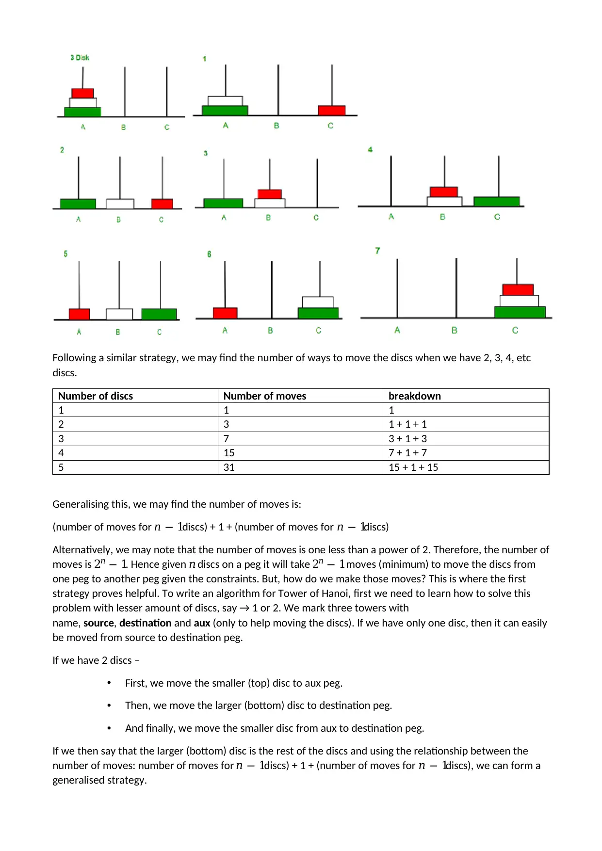
Approach:
• Recursively Move N-1 disc from source to Auxiliary peg.
• Move the last disc from source to destination.
• Recursively Move N-1 disc from Auxiliary to destination peg
The steps to follow are:
Step 1 − Move n-1 discs from source to aux
Step 2 − Move nth disc from source to dest
Step 3 − Move n-1 discs from aux to dest
From which we can produce pseudo-code to solve the Towers of Hanoi
problem.
START Procedure Hanoi(disc, source, dest, aux)
IF disc == 1, THEN
move disc from source to dest
ELSE
Hanoi(disc - 1, source, aux, dest) // Step 1
move disc from source to dest // Step 2
Hanoi(disc - 1, aux, dest, source) // Step 3
END IF
END Procedure STOP
Which, in Python, is:
def TowerOfHanoi(n , source, destination, auxiliary):
if n==1:
print ("Move disc 1 from source",source,"to destination",destination)
return
TowerOfHanoi(n-1, source, auxiliary, destination)
print ("Move disc",n,"from source",source,"to destination",destination)
TowerOfHanoi(n-1, auxiliary, destination, source)
# test code
n = 4
TowerOfHanoi(n,'A','B','C')
# A, C, B are the name of rods
To test this, we may look at the solutions or prove it via induction.
For the Tower of Hanoi, we have the number of moves, 𝑆𝑛 is 𝑆𝑛 = 2𝑛 − 1for 𝑛 discs, this is our 𝑃(𝑛).
Paraphrase This Document
Need a fresh take? Get an instant paraphrase of this document with our AI Paraphraser
Base case, 𝑃(1): 𝑆1 = 21 − 1 = 2 − 1 = 1. We know it takes one move to move one disc, so 𝑃(1)is true.
We assume that 𝑃(𝑘): 𝑆𝑘 = 2𝑘 − 1is true.
Now, for 𝑃(𝑘 + 1): 𝑆𝑘+1 = 2𝑘+1 − 1
𝑆𝑘+1 = (𝑛𝑢𝑚𝑏𝑒𝑟 𝑜𝑓 𝑚𝑜𝑣𝑒𝑠 𝑟𝑒𝑞𝑢𝑖𝑟𝑒𝑑 𝑡𝑜 𝑚𝑜𝑣𝑒 𝑘 𝑑𝑖𝑠𝑐𝑠 𝑜𝑓 𝑡ℎ𝑒 𝑏𝑜𝑡𝑡𝑜𝑚 𝑑𝑖𝑠𝑘)
+ (1 𝑚𝑜𝑣𝑒 𝑡𝑜 𝑚𝑜𝑣𝑒 𝑡ℎ𝑒 𝑏𝑎𝑠𝑒 𝑑𝑖𝑠𝑐)
+ (𝑛𝑢𝑚𝑏𝑒𝑟 𝑜𝑓 𝑚𝑜𝑣𝑒𝑠 𝑟𝑒𝑞𝑢𝑖𝑟𝑒𝑑 𝑡𝑜 𝑚𝑜𝑣𝑒 𝑡ℎ𝑒 𝑘 𝑑𝑖𝑠𝑐𝑠 𝑏𝑎𝑐𝑘 𝑜𝑛𝑡𝑜 𝑡ℎ𝑒 𝑏𝑎𝑠𝑒 𝑑𝑖
= 𝑆𝑘 + 1 + 𝑆𝑘 = 2𝑆𝑘 + 1 = 2(2𝑘 − 1) + 1
= 2 × 2𝑘 − 2 + 1 = 21 × 2𝑘 − 1 = 2𝑘+1 − 1
Hence 𝑃(𝑘 + 1) is true provided that 𝑃(𝑘)is true.
Therefore, by mathematical induction, the number of moves for the Tower of Hanoi is 𝑆𝑛 = 2𝑛 − 1
We therefore have the number of moves is 2𝑛 − 1. We note that:
𝑆1 = 1
𝑆2 = 3 = 2 × 1 + 1 = 2𝑆1 + 1
𝑆3 = 7 = 2 × 3 + 1 = 2𝑆2 + 1
𝑆4 = 15 = 2 × 7 + 1 = 2𝑆3 + 1
By looking at the pattern, we have
𝑆𝑛 = 2𝑆𝑛−1 + 1, 𝑆1 = 1
As our recursive formula.
Assessing the result:
Our solutions meets the requirements, we have found the minimal number of moves and how to make those
moves using recursion. We can then test the algorithm on 2 discs and 3 discs, etc and we get the correct
number of moves as well as the method to achieve those moves.
We could possibly make some aspects easier; however, the most simple solution in this case is the recursive
approach
Describing what we have learnt:
We learnt that we can use recursion to help solve problems and strengthen the idea of breaking a problem up
to look at simpler cases before generalising.
This problem was difficult in that the approach used is different to the noughts and crosses problem due to
the increased complexity of the solution and the exponential nature of number of moves rather than the
quadratic nature.
Documenting the solution:
Reread our solution, is there anything that should be rewritten?
Not in this case, we cannot see anything that is difficult to understand
Recurrence Relations
We have already met recurrence relations, although not formally defined what they are. Consider the
following instructions for generating a sequence:
1. Start with 5
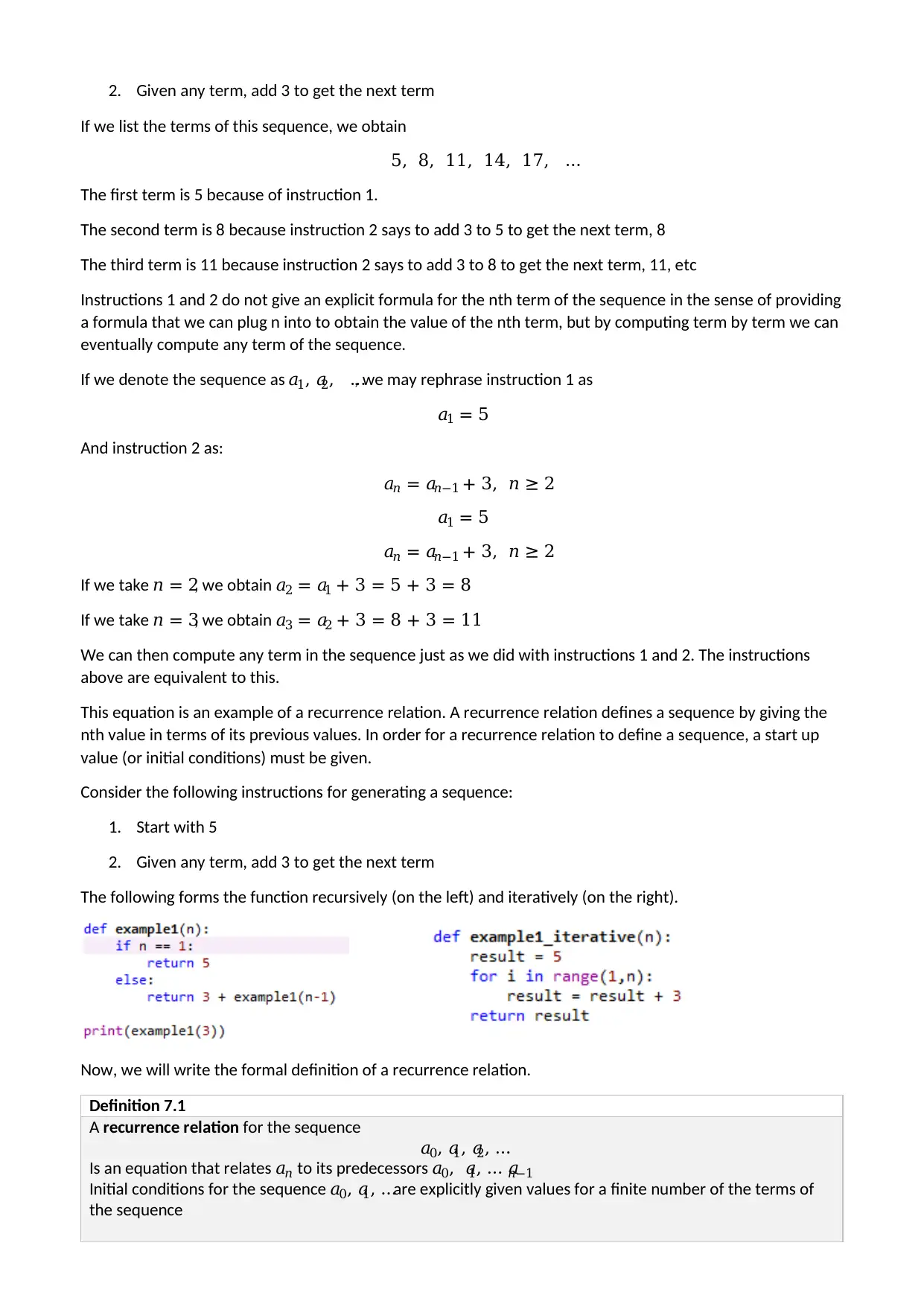
2. Given any term, add 3 to get the next term
If we list the terms of this sequence, we obtain
5, 8, 11, 14, 17, …
The first term is 5 because of instruction 1.
The second term is 8 because instruction 2 says to add 3 to 5 to get the next term, 8
The third term is 11 because instruction 2 says to add 3 to 8 to get the next term, 11, etc
Instructions 1 and 2 do not give an explicit formula for the nth term of the sequence in the sense of providing
a formula that we can plug n into to obtain the value of the nth term, but by computing term by term we can
eventually compute any term of the sequence.
If we denote the sequence as 𝑎1, 𝑎2, …, we may rephrase instruction 1 as
𝑎1 = 5
And instruction 2 as:
𝑎𝑛 = 𝑎𝑛−1 + 3, 𝑛 ≥ 2
𝑎1 = 5
𝑎𝑛 = 𝑎𝑛−1 + 3, 𝑛 ≥ 2
If we take 𝑛 = 2, we obtain 𝑎2 = 𝑎1 + 3 = 5 + 3 = 8
If we take 𝑛 = 3, we obtain 𝑎3 = 𝑎2 + 3 = 8 + 3 = 11
We can then compute any term in the sequence just as we did with instructions 1 and 2. The instructions
above are equivalent to this.
This equation is an example of a recurrence relation. A recurrence relation defines a sequence by giving the
nth value in terms of its previous values. In order for a recurrence relation to define a sequence, a start up
value (or initial conditions) must be given.
Consider the following instructions for generating a sequence:
1. Start with 5
2. Given any term, add 3 to get the next term
The following forms the function recursively (on the left) and iteratively (on the right).
Now, we will write the formal definition of a recurrence relation.
Definition 7.1
A recurrence relation for the sequence
𝑎0, 𝑎1, 𝑎2, …
Is an equation that relates 𝑎𝑛 to its predecessors 𝑎0, 𝑎1, … 𝑎𝑛−1
Initial conditions for the sequence 𝑎0, 𝑎1, …are explicitly given values for a finite number of the terms of
the sequence
⊘ This is a preview!⊘
Do you want full access?
Subscribe today to unlock all pages.
Trusted by 1+ million students worldwide
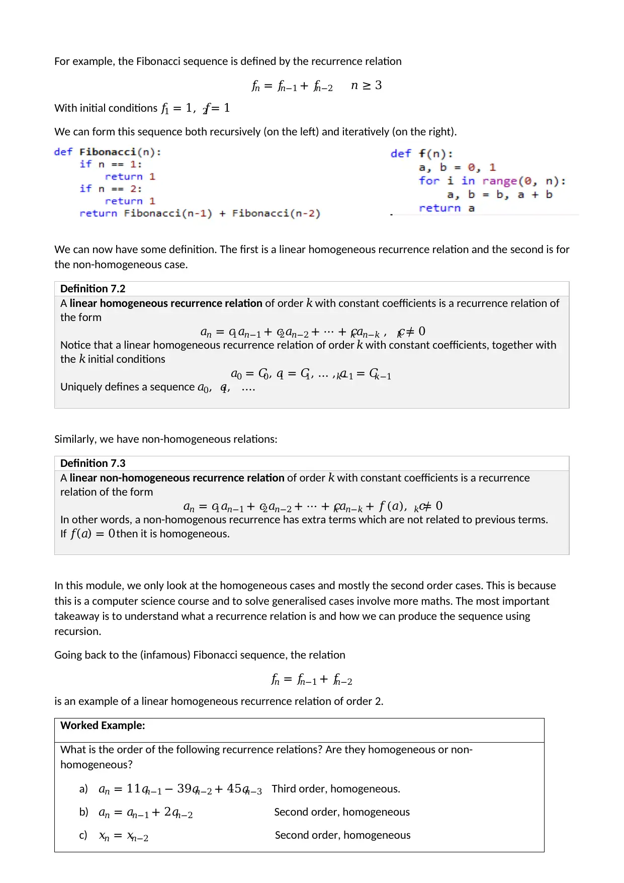
For example, the Fibonacci sequence is defined by the recurrence relation
𝑓𝑛 = 𝑓𝑛−1 + 𝑓𝑛−2 𝑛 ≥ 3
With initial conditions 𝑓1 = 1, 𝑓2 = 1
We can form this sequence both recursively (on the left) and iteratively (on the right).
We can now have some definition. The first is a linear homogeneous recurrence relation and the second is for
the non-homogeneous case.
Definition 7.2
A linear homogeneous recurrence relation of order 𝑘 with constant coefficients is a recurrence relation of
the form
𝑎𝑛 = 𝑐1𝑎𝑛−1 + 𝑐2𝑎𝑛−2 + ⋯ + 𝑐𝑘𝑎𝑛−𝑘 , 𝑐𝑘 ≠ 0
Notice that a linear homogeneous recurrence relation of order 𝑘 with constant coefficients, together with
the 𝑘 initial conditions
𝑎0 = 𝐶0, 𝑎1 = 𝐶1, … , 𝑎𝑘−1 = 𝐶𝑘−1
Uniquely defines a sequence 𝑎0, 𝑎1, ….
Similarly, we have non-homogeneous relations:
Definition 7.3
A linear non-homogeneous recurrence relation of order 𝑘 with constant coefficients is a recurrence
relation of the form
𝑎𝑛 = 𝑐1𝑎𝑛−1 + 𝑐2𝑎𝑛−2 + ⋯ + 𝑐𝑘𝑎𝑛−𝑘 + 𝑓(𝑎), 𝑐𝑘 ≠ 0
In other words, a non-homogenous recurrence has extra terms which are not related to previous terms.
If 𝑓(𝑎) = 0 then it is homogeneous.
In this module, we only look at the homogeneous cases and mostly the second order cases. This is because
this is a computer science course and to solve generalised cases involve more maths. The most important
takeaway is to understand what a recurrence relation is and how we can produce the sequence using
recursion.
Going back to the (infamous) Fibonacci sequence, the relation
𝑓𝑛 = 𝑓𝑛−1 + 𝑓𝑛−2
is an example of a linear homogeneous recurrence relation of order 2.
Worked Example:
What is the order of the following recurrence relations? Are they homogeneous or non-
homogeneous?
a) 𝑎𝑛 = 11𝑎𝑛−1 − 39𝑎𝑛−2 + 45𝑎𝑛−3 Third order, homogeneous.
b) 𝑎𝑛 = 𝑎𝑛−1 + 2𝑎𝑛−2 Second order, homogeneous
c) 𝑥𝑛 = 𝑥𝑛−2 Second order, homogeneous
Paraphrase This Document
Need a fresh take? Get an instant paraphrase of this document with our AI Paraphraser
d) 𝑎𝑛 = 𝑎𝑛−1 + 4 First order, non-homogeneous
e) 𝑎𝑛 = 5𝑎𝑛−1 − 4𝑎𝑛−2 + 𝑛2 Second order, non-homogeneous.
Your turn:
What is the order of the following recurrence relations? Are they homogeneous or non-
homogeneous?
a) 𝑎𝑛 = 3𝑎𝑛−1 + 𝑎𝑛−2 + 𝑎𝑛−4
b) 𝑎𝑛 = 5𝑎𝑛−1 − 3𝑎𝑛−2 − 1
Second Order Linear Homogeneous Recurrence Relations
Let
𝑎𝑛 = 𝑐1𝑎𝑛−1 + 𝑐2𝑎𝑛−2
Be a second order, linear homogeneous recurrence relation with constant coefficients.
If 𝑆and 𝑇are solutions, then 𝑈 = 𝑏𝑆 + 𝑑𝑇is also a solution of *.
If 𝑟 is a root of the characteristic (or auxiliary) equation defined as:
𝑡2 − 𝑐1𝑡 − 𝑐2 = 0
Then the sequence 𝑟𝑛, 𝑛 = 0,1, …is a solution. If 𝑎 is the sequence defined by *,
𝑎0 = 𝐶0, 𝑎1 = 𝐶1
And 𝑟1 and 𝑟2 are roots of * with 𝑟1 ≠ 𝑟2, then there exist constants 𝑏 and 𝑑 such that
𝑎𝑛 = 𝑏𝑟1
𝑛 + 𝑑𝑟2
𝑛
This is called the general solution.
Given a set of initial conditions, finding the values of 𝑏 and 𝑑 result in the particular solution.
Worked Example:
What is the general and particular solutions to the recurrence relation 𝑎𝑛 = 7𝑎𝑛−1 − 12𝑎𝑛−2 with
initial conditions 𝑎1 = 1 and 𝑎2 = 4?
Rearranging gives:
Therefore, the characteristic solution is:
𝑡2 − 7𝑡 + 12 = 0
This can be factorised as
(𝑡 − 4)(𝑡 − 3) = 0
And has solutions 𝑡 = 4and 𝑡 = 3. Therefore, the general solution is
𝑎𝑛 = 𝑏 × 4𝑛 + 𝑑 × 3𝑛
Substituting the first two values in 𝑎1 = 1 and 𝑎2 = 4 gives
𝑎1: 1 = 4𝑏 + 3𝑑
𝑎2: 4 = 16𝑏 + 9𝑑
Solving these simultaneous equations gives the solution 𝑏 =1
4 and 𝑑 = 0.
Therefore, the particular solution is 𝑎𝑛 = 1
4 × 4𝑛 + 0 × 3𝑛 = 1
4 × 4𝑛 or 𝑎𝑛 = 4𝑛−1
Your turn:
What is the general and particular solutions to the recurrence relation 𝑎𝑛 = 7𝑎𝑛−1 − 12𝑎𝑛−2 with
initial conditions 𝑎1 = 1 and 𝑎2 = 3
Application: Fibonacci and Lucas Recurrence Relations
The relation
𝑓𝑛 = 𝑓𝑛−1 + 𝑓𝑛−2
Can be rewritten as 𝑓𝑛 − 𝑓𝑛−1 − 𝑓𝑛−2, 𝑛 ≥ 3and initial conditions 𝑓1 = 1, 𝑓2 = 1.
We begin by using the quadratic formula to solve
𝑡2 − 𝑡 − 1 = 0
The solution of this quadratic is 𝑡 =1±√5
2
𝑡 =1 ±√5
2
Thus, the general solution is:
𝑓𝑛 = 𝑏( 1 +√5
2 )
𝑛
+ 𝑑( 1 −√5
2 )
𝑛
To find the particular solution:
𝑓𝑛 = 𝑏( 1 +√5
2 )
𝑛
+ 𝑑( 1 −√5
2 )
𝑛
To satisfy the initial conditions, we must have
𝑏( 1 +√5
2 ) + 𝑑( 1 −√5
2 ) = 1
And
𝑏( 1 +√5
2 )
2
+ 𝑑( 1 −√5
2 )
2
= 1
𝑓𝑛 = 𝑏( 1 +√5
2 )
𝑛
+ 𝑑( 1 −√5
2 )
𝑛
Using the initial conditions and the first term of the sequence, we have:
⊘ This is a preview!⊘
Do you want full access?
Subscribe today to unlock all pages.
Trusted by 1+ million students worldwide
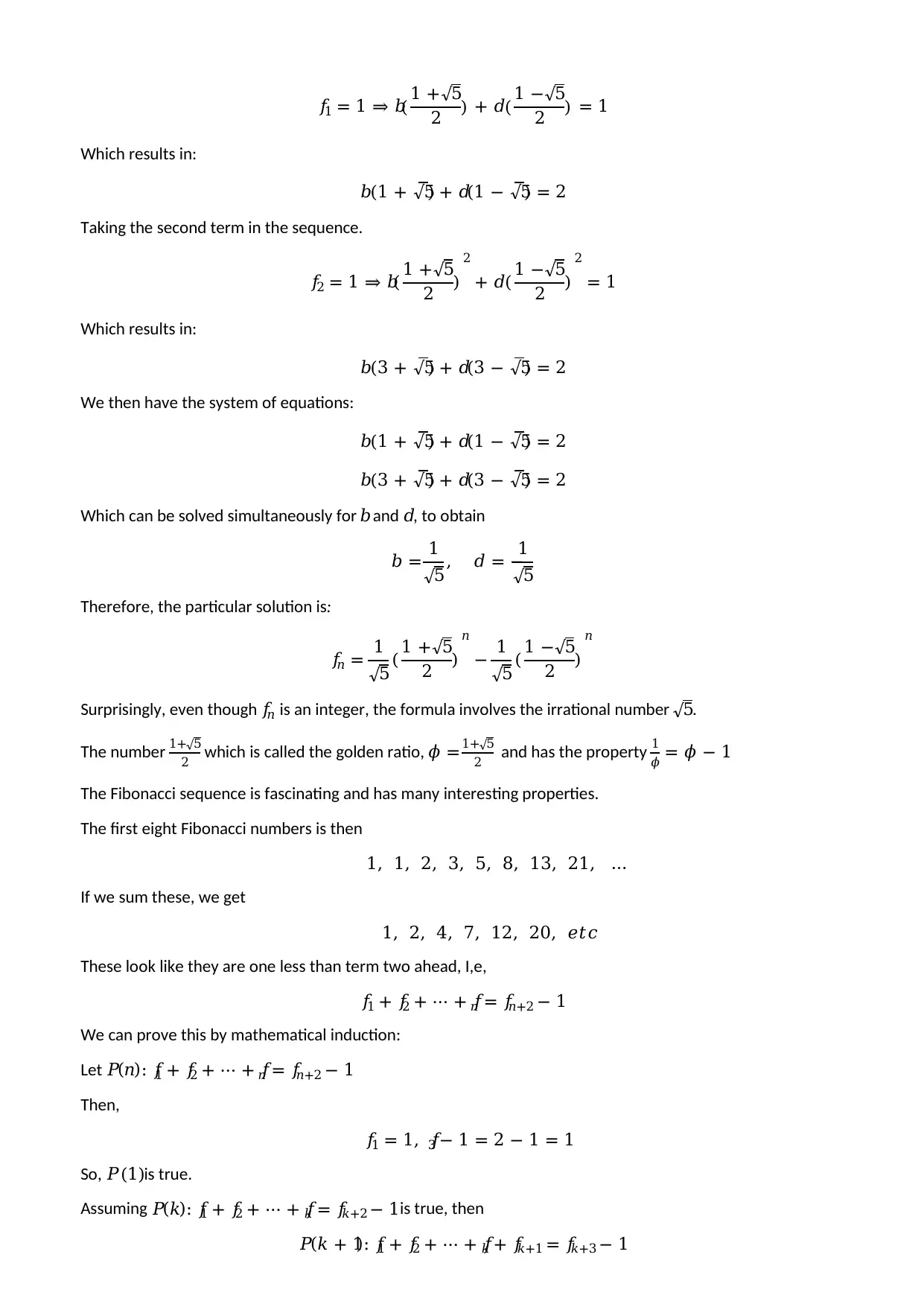
𝑓1 = 1 ⇒ 𝑏( 1 +√5
2 ) + 𝑑( 1 −√5
2 ) = 1
Which results in:
𝑏(1 + √5) + 𝑑(1 − √5) = 2
Taking the second term in the sequence.
𝑓2 = 1 ⇒ 𝑏( 1 +√5
2 )
2
+ 𝑑( 1 −√5
2 )
2
= 1
Which results in:
𝑏(3 + √5) + 𝑑(3 − √5) = 2
We then have the system of equations:
𝑏(1 + √5) + 𝑑(1 − √5) = 2
𝑏(3 + √5) + 𝑑(3 − √5) = 2
Which can be solved simultaneously for 𝑏 and 𝑑, to obtain
𝑏 = 1
√5, 𝑑 = −
1
√5
Therefore, the particular solution is:
𝑓𝑛 = 1
√5( 1 +√5
2 )
𝑛
− 1
√5( 1 −√5
2 )
𝑛
Surprisingly, even though 𝑓𝑛 is an integer, the formula involves the irrational number √5.
The number 1+√5
2 which is called the golden ratio, 𝜙 = 1+√5
2 and has the property 1
𝜙 = 𝜙 − 1.
The Fibonacci sequence is fascinating and has many interesting properties.
The first eight Fibonacci numbers is then
1, 1, 2, 3, 5, 8, 13, 21, …
If we sum these, we get
1, 2, 4, 7, 12, 20, 𝑒𝑡𝑐
These look like they are one less than term two ahead, I,e,
𝑓1 + 𝑓2 + ⋯ + 𝑓𝑛 = 𝑓𝑛+2 − 1
We can prove this by mathematical induction:
Let 𝑃(𝑛): 𝑓1 + 𝑓2 + ⋯ + 𝑓𝑛 = 𝑓𝑛+2 − 1
Then,
𝑓1 = 1, 𝑓3 − 1 = 2 − 1 = 1
So, 𝑃(1)is true.
Assuming 𝑃(𝑘): 𝑓1 + 𝑓2 + ⋯ + 𝑓𝑘 = 𝑓𝑘+2 − 1is true, then
𝑃(𝑘 + 1): 𝑓1 + 𝑓2 + ⋯ + 𝑓𝑘 + 𝑓𝑘+1 = 𝑓𝑘+3 − 1
Paraphrase This Document
Need a fresh take? Get an instant paraphrase of this document with our AI Paraphraser
Now, as 𝑃(𝑘)is true
𝑓𝑘+2 − 1 + 𝑓𝑘+1 = 𝑓𝑘+3 − 1
As 𝑓𝑘+1 + 𝑓𝑘+2 = 𝑓𝑘+3 by definition. Therefore 𝑃(𝑘 + 1)is true. Therefore, by mathematical induction, as
𝑃(𝑘) → 𝑃(𝑘 + 1)is true and 𝑃(1)is true, then
𝑓1 + 𝑓2 + ⋯ + 𝑓𝑛 = 𝑓𝑛+2 − 1
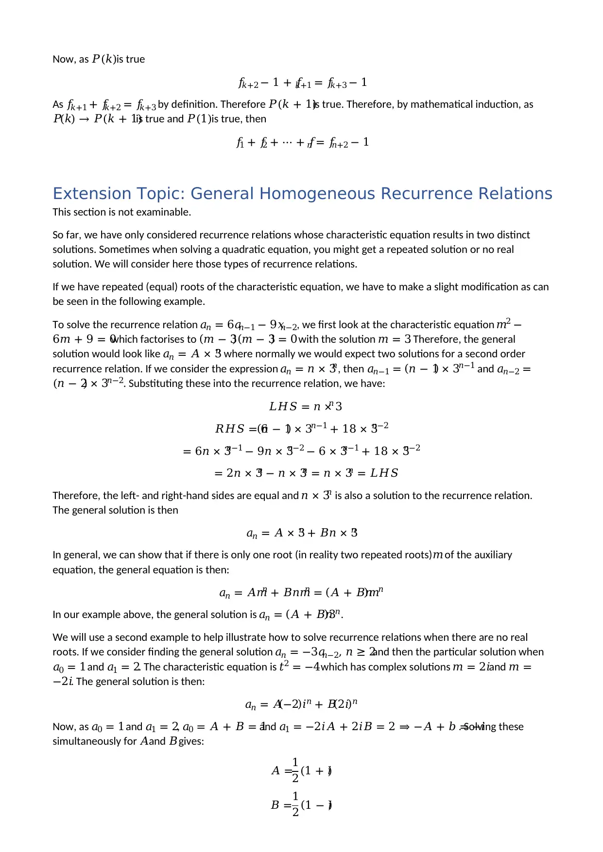
Extension Topic: General Homogeneous Recurrence Relations
This section is not examinable.
So far, we have only considered recurrence relations whose characteristic equation results in two distinct
solutions. Sometimes when solving a quadratic equation, you might get a repeated solution or no real
solution. We will consider here those types of recurrence relations.
If we have repeated (equal) roots of the characteristic equation, we have to make a slight modification as can
be seen in the following example.
To solve the recurrence relation 𝑎𝑛 = 6𝑎𝑛−1 − 9𝑥𝑛−2, we first look at the characteristic equation 𝑚2 −
6𝑚 + 9 = 0which factorises to (𝑚 − 3)(𝑚 − 3) = 0 with the solution 𝑚 = 3. Therefore, the general
solution would look like 𝑎𝑛 = 𝐴 × 3𝑛 where normally we would expect two solutions for a second order
recurrence relation. If we consider the expression 𝑎𝑛 = 𝑛 × 3𝑛, then 𝑎𝑛−1 = (𝑛 − 1) × 3𝑛−1 and 𝑎𝑛−2 =
(𝑛 − 2) × 3𝑛−2. Substituting these into the recurrence relation, we have:
𝐿𝐻𝑆 = 𝑛 × 3𝑛
𝑅𝐻𝑆 = 6(𝑛 − 1) × 3𝑛−1 + 18 × 3𝑛−2
= 6𝑛 × 3𝑛−1 − 9𝑛 × 3𝑛−2 − 6 × 3𝑛−1 + 18 × 3𝑛−2
= 2𝑛 × 3𝑛 − 𝑛 × 3𝑛 = 𝑛 × 3𝑛 = 𝐿𝐻𝑆
Therefore, the left- and right-hand sides are equal and 𝑛 × 3𝑛 is also a solution to the recurrence relation.
The general solution is then
𝑎𝑛 = 𝐴 × 3𝑛 + 𝐵𝑛 × 3𝑛
In general, we can show that if there is only one root (in reality two repeated roots) 𝑚 of the auxiliary
equation, the general equation is then:
𝑎𝑛 = 𝐴𝑚𝑛 + 𝐵𝑛𝑚𝑛 = (𝐴 + 𝐵𝑛)𝑚𝑛
In our example above, the general solution is 𝑎𝑛 = (𝐴 + 𝐵𝑛)3𝑛.
We will use a second example to help illustrate how to solve recurrence relations when there are no real
roots. If we consider finding the general solution 𝑎𝑛 = −3𝑎𝑛−2, 𝑛 ≥ 2and then the particular solution when
𝑎0 = 1 and 𝑎1 = 2. The characteristic equation is 𝑡2 = −4which has complex solutions 𝑚 = 2𝑖and 𝑚 =
−2𝑖. The general solution is then:
𝑎𝑛 = 𝐴(−2)𝑖𝑛 + 𝐵(2𝑖)𝑛
Now, as 𝑎0 = 1 and 𝑎1 = 2, 𝑎0 = 𝐴 + 𝐵 = 1and 𝑎1 = −2𝑖𝐴 + 2𝑖𝐵 = 2 ⇒ −𝐴 + 𝑏 = −𝑖. Solving these
simultaneously for 𝐴and 𝐵 gives:
𝐴 =1
2(1 + 𝑖)
𝐵 =1
2(1 − 𝑖)
𝑓𝑘+2 − 1 + 𝑓𝑘+1 = 𝑓𝑘+3 − 1
As 𝑓𝑘+1 + 𝑓𝑘+2 = 𝑓𝑘+3 by definition. Therefore 𝑃(𝑘 + 1)is true. Therefore, by mathematical induction, as
𝑃(𝑘) → 𝑃(𝑘 + 1)is true and 𝑃(1)is true, then
𝑓1 + 𝑓2 + ⋯ + 𝑓𝑛 = 𝑓𝑛+2 − 1
Extension Topic: General Homogeneous Recurrence Relations
This section is not examinable.
So far, we have only considered recurrence relations whose characteristic equation results in two distinct
solutions. Sometimes when solving a quadratic equation, you might get a repeated solution or no real
solution. We will consider here those types of recurrence relations.
If we have repeated (equal) roots of the characteristic equation, we have to make a slight modification as can
be seen in the following example.
To solve the recurrence relation 𝑎𝑛 = 6𝑎𝑛−1 − 9𝑥𝑛−2, we first look at the characteristic equation 𝑚2 −
6𝑚 + 9 = 0which factorises to (𝑚 − 3)(𝑚 − 3) = 0 with the solution 𝑚 = 3. Therefore, the general
solution would look like 𝑎𝑛 = 𝐴 × 3𝑛 where normally we would expect two solutions for a second order
recurrence relation. If we consider the expression 𝑎𝑛 = 𝑛 × 3𝑛, then 𝑎𝑛−1 = (𝑛 − 1) × 3𝑛−1 and 𝑎𝑛−2 =
(𝑛 − 2) × 3𝑛−2. Substituting these into the recurrence relation, we have:
𝐿𝐻𝑆 = 𝑛 × 3𝑛
𝑅𝐻𝑆 = 6(𝑛 − 1) × 3𝑛−1 + 18 × 3𝑛−2
= 6𝑛 × 3𝑛−1 − 9𝑛 × 3𝑛−2 − 6 × 3𝑛−1 + 18 × 3𝑛−2
= 2𝑛 × 3𝑛 − 𝑛 × 3𝑛 = 𝑛 × 3𝑛 = 𝐿𝐻𝑆
Therefore, the left- and right-hand sides are equal and 𝑛 × 3𝑛 is also a solution to the recurrence relation.
The general solution is then
𝑎𝑛 = 𝐴 × 3𝑛 + 𝐵𝑛 × 3𝑛
In general, we can show that if there is only one root (in reality two repeated roots) 𝑚 of the auxiliary
equation, the general equation is then:
𝑎𝑛 = 𝐴𝑚𝑛 + 𝐵𝑛𝑚𝑛 = (𝐴 + 𝐵𝑛)𝑚𝑛
In our example above, the general solution is 𝑎𝑛 = (𝐴 + 𝐵𝑛)3𝑛.
We will use a second example to help illustrate how to solve recurrence relations when there are no real
roots. If we consider finding the general solution 𝑎𝑛 = −3𝑎𝑛−2, 𝑛 ≥ 2and then the particular solution when
𝑎0 = 1 and 𝑎1 = 2. The characteristic equation is 𝑡2 = −4which has complex solutions 𝑚 = 2𝑖and 𝑚 =
−2𝑖. The general solution is then:
𝑎𝑛 = 𝐴(−2)𝑖𝑛 + 𝐵(2𝑖)𝑛
Now, as 𝑎0 = 1 and 𝑎1 = 2, 𝑎0 = 𝐴 + 𝐵 = 1and 𝑎1 = −2𝑖𝐴 + 2𝑖𝐵 = 2 ⇒ −𝐴 + 𝑏 = −𝑖. Solving these
simultaneously for 𝐴and 𝐵 gives:
𝐴 =1
2(1 + 𝑖)
𝐵 =1
2(1 − 𝑖)
The particular solution is 𝑎𝑛 = 1
2 (1 + 𝑖)(−2𝑖)𝑛 + 1
2 (1 − 𝑖)(2𝑖)𝑛.
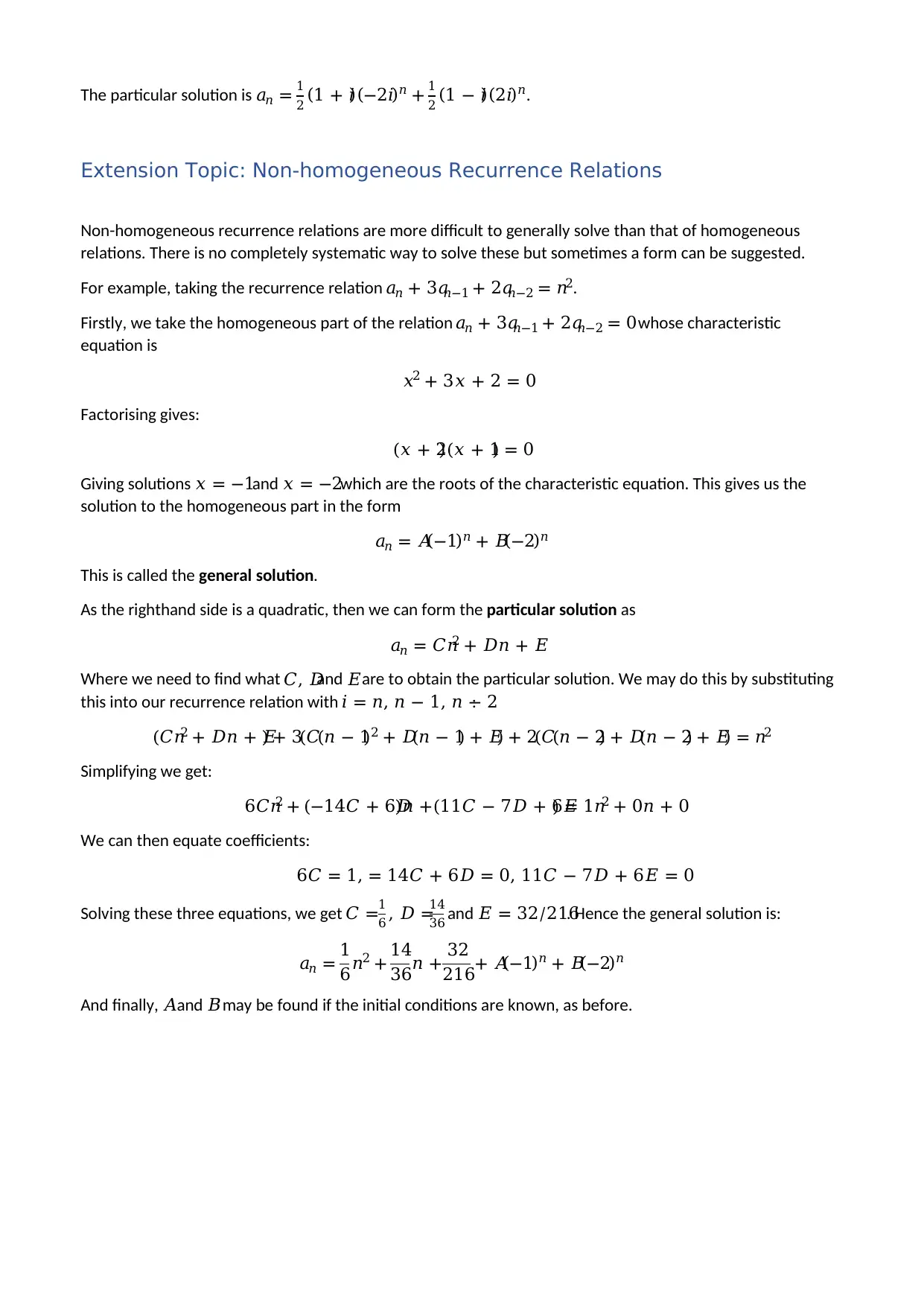
Extension Topic: Non-homogeneous Recurrence Relations
Non-homogeneous recurrence relations are more difficult to generally solve than that of homogeneous
relations. There is no completely systematic way to solve these but sometimes a form can be suggested.
For example, taking the recurrence relation 𝑎𝑛 + 3𝑎𝑛−1 + 2𝑎𝑛−2 = 𝑛2.
Firstly, we take the homogeneous part of the relation 𝑎𝑛 + 3𝑎𝑛−1 + 2𝑎𝑛−2 = 0 whose characteristic
equation is
𝑥2 + 3𝑥 + 2 = 0
Factorising gives:
(𝑥 + 2)(𝑥 + 1) = 0
Giving solutions 𝑥 = −1and 𝑥 = −2which are the roots of the characteristic equation. This gives us the
solution to the homogeneous part in the form
𝑎𝑛 = 𝐴(−1)𝑛 + 𝐵(−2)𝑛
This is called the general solution.
As the righthand side is a quadratic, then we can form the particular solution as
𝑎𝑛 = 𝐶𝑛2 + 𝐷𝑛 + 𝐸
Where we need to find what 𝐶, 𝐷and 𝐸are to obtain the particular solution. We may do this by substituting
this into our recurrence relation with 𝑖 = 𝑛, 𝑛 − 1, 𝑛 − 2:
(𝐶𝑛2 + 𝐷𝑛 + 𝐸) + 3(𝐶(𝑛 − 1)2 + 𝐷(𝑛 − 1) + 𝐸) + 2(𝐶(𝑛 − 2) + 𝐷(𝑛 − 2) + 𝐸) = 𝑛2
Simplifying we get:
6𝐶𝑛2 + (−14𝐶 + 6𝐷)𝑛 +(11𝐶 − 7𝐷 + 6𝐸) = 1𝑛2 + 0𝑛 + 0
We can then equate coefficients:
6𝐶 = 1, = 14𝐶 + 6𝐷 = 0, 11𝐶 − 7𝐷 + 6𝐸 = 0
Solving these three equations, we get 𝐶 =1
6 , 𝐷 =
14
36 and 𝐸 = 32/216. Hence the general solution is:
𝑎𝑛 = 1
6𝑛2 + 14
36𝑛 + 32
216+ 𝐴(−1)𝑛 + 𝐵(−2)𝑛
And finally, 𝐴and 𝐵 may be found if the initial conditions are known, as before.
2 (1 + 𝑖)(−2𝑖)𝑛 + 1
2 (1 − 𝑖)(2𝑖)𝑛.
Extension Topic: Non-homogeneous Recurrence Relations
Non-homogeneous recurrence relations are more difficult to generally solve than that of homogeneous
relations. There is no completely systematic way to solve these but sometimes a form can be suggested.
For example, taking the recurrence relation 𝑎𝑛 + 3𝑎𝑛−1 + 2𝑎𝑛−2 = 𝑛2.
Firstly, we take the homogeneous part of the relation 𝑎𝑛 + 3𝑎𝑛−1 + 2𝑎𝑛−2 = 0 whose characteristic
equation is
𝑥2 + 3𝑥 + 2 = 0
Factorising gives:
(𝑥 + 2)(𝑥 + 1) = 0
Giving solutions 𝑥 = −1and 𝑥 = −2which are the roots of the characteristic equation. This gives us the
solution to the homogeneous part in the form
𝑎𝑛 = 𝐴(−1)𝑛 + 𝐵(−2)𝑛
This is called the general solution.
As the righthand side is a quadratic, then we can form the particular solution as
𝑎𝑛 = 𝐶𝑛2 + 𝐷𝑛 + 𝐸
Where we need to find what 𝐶, 𝐷and 𝐸are to obtain the particular solution. We may do this by substituting
this into our recurrence relation with 𝑖 = 𝑛, 𝑛 − 1, 𝑛 − 2:
(𝐶𝑛2 + 𝐷𝑛 + 𝐸) + 3(𝐶(𝑛 − 1)2 + 𝐷(𝑛 − 1) + 𝐸) + 2(𝐶(𝑛 − 2) + 𝐷(𝑛 − 2) + 𝐸) = 𝑛2
Simplifying we get:
6𝐶𝑛2 + (−14𝐶 + 6𝐷)𝑛 +(11𝐶 − 7𝐷 + 6𝐸) = 1𝑛2 + 0𝑛 + 0
We can then equate coefficients:
6𝐶 = 1, = 14𝐶 + 6𝐷 = 0, 11𝐶 − 7𝐷 + 6𝐸 = 0
Solving these three equations, we get 𝐶 =1
6 , 𝐷 =
14
36 and 𝐸 = 32/216. Hence the general solution is:
𝑎𝑛 = 1
6𝑛2 + 14
36𝑛 + 32
216+ 𝐴(−1)𝑛 + 𝐵(−2)𝑛
And finally, 𝐴and 𝐵 may be found if the initial conditions are known, as before.
⊘ This is a preview!⊘
Do you want full access?
Subscribe today to unlock all pages.
Trusted by 1+ million students worldwide
1 out of 20


Your All-in-One AI-Powered Toolkit for Academic Success.
+13062052269
info@desklib.com
Available 24*7 on WhatsApp / Email
![[object Object]](/_next/static/media/star-bottom.7253800d.svg)
Unlock your academic potential
Copyright © 2020–2026 A2Z Services. All Rights Reserved. Developed and managed by ZUCOL.