Regression Analysis: Examining Tax and Deregulation Impact
VerifiedAdded on 2023/06/11
|16
|1898
|150
Homework Assignment
AI Summary
This assignment delves into several key econometric concepts and applies them to analyze economic policies. It begins by explaining the importance of endogenous sample selection, errors in variables, and strict exogeneity in regression models. The assignment then explores the usefulness of introducing deregulation policies at different times for different companies when conducting a difference-in-difference analysis. Furthermore, it examines the long-run effect of personal tax exemptions on fertility rates, including hypothesis testing and interpretation of results. The study also includes a detailed statistical analysis of variables like 'countercyc,' 'cagpb_fd,' and 'output_gap_fd,' including stationarity tests, unit root tests, and regressions on market economy indicators and financial market variables. Finally, the assignment investigates correlation and regression analyses with simulated data, focusing on spurious regressions and the use of time trends to address persistence issues. The document provides comprehensive insights into econometric modeling and policy evaluation. Desklib offers a platform to access this and similar solved assignments, enhancing students' understanding and academic performance.

Question one
i. Endogenous sample selection
Endogeinity arises from the wrong identification of the causal relationship between
factors say X and Z where in the real sense the relationship that was observed was
between caused by a different factor say Y. Endogenous sample selection occurs
when selection into the sample is based on the dependent variable. Often endogenous
sample selection leads to bias and inconsistency of the selected sample parameters.
ii. Errors in variables
They occur due to wrong measurement of variables that may be caused by factors
such as imprecise recording or wrong proxy variables in the financial regression
model, (Maddala and Nimalendran, 1996) . They often have a mean of zero hence do
not affect the response variables but tend to occur in the error term of a regression
model if the predictor variables are measured with error. As such errors in variables
do cause problems in financial models when measuring factors that influence or cause
the response variables.
iii. Strict exogeneity
When the error term is uncorrelated with all dummy variables i.e. with past and future
dummy variables it is referred to as strict exogeneity. Implying the variable are
nonreactive to past and future shocks.
Paraphrase This Document
Need a fresh take? Get an instant paraphrase of this document with our AI Paraphraser

Question two
i. Usefulness of introducing deregulation policy on company prices at different
points in time.
Generally, DID is a quasi-experiment that utilizing longitudinal information from
control and treatment groups seek to get suitable counter-factual for estimating the
causal-effect. When projecting the effect deregulation on company prices we compare
the performance of company prices before and after introduction of the policy, in the
process, we make the “parallel paths “ assumption which suggests that, “average
change in comparison group represent counter-factual change in treatment group if
there were no treatment.” DID also assumes that, “in case of absence of treatment, the
unobserved differences between treatment and control groups is the sames over time”
(Columbia University, 2016). Using panel data from different times, we examine for
the assumption by conducting a test for differences in all pre-treatment trends for
comparison and treatment groups. Introducing the policy in different times for
different company would help in the outcome of one company acting a control for the
other company. Since the “parallel paths” assumption has no statistical tests it relies in
intuition and observation and thus has potential limitations such as:
i. It is not applicable if the future and past groups composition are unstable
ii. Not suitable if the groups to be compared have different outcome trend
Introducing the policy at different times for different groups would also enable per-
determination of the outcome trend from each company and enable us use a different
approach when applying it to a different company so as to obtain correct observation
of the causal effect.

Question three
i. Estimated long-run effect of personal tax exemption on fertility
The effect of tax exemption is estimated to be positive at 7.3% while the long-run
effect is (0.073-0.0058+0.0034=0.1012), hence 10.12% long run effect of tax
exemption on fertility
Interpretation
Given a 10.12% we deduce that tax exemption lowers the cost of raising children and
therefore leads to more demand of children, while holding all other factors constant.
ii. Testing Hypotheses
H0: Personal tax exemption has no effect on fertility
H1: Personal tax exemption has got effect on fertility
Test
At a significance level of 0.05, the F-statistic has a P-value of 0.12 which is greater
than 0.05. We therefore reject the null hypothesis that personal tax exemption has no
effect on fertility and accept the alternative hypothesis that tax has effect on fertility.
And hence conclude that tax exemption does have effect on fertility.
iii. Explanation of the outcome of the hypothesis test in relation to significance
of individual coefficients
At a 1% significance level, each of the response variables are individually
insignificant, partially due to estimation. However the three explanatory variables are
assumed to be jointly significant also as can be deduced from the test of hypothesis
that tax exemption has effect on fertility rates.
⊘ This is a preview!⊘
Do you want full access?
Subscribe today to unlock all pages.

Trusted by 1+ million students worldwide
(i) We can therefore conclude that the three explanatory jointly influence the fertility
rate of one birth per 1000 women of childbearing age.
Question 4
i. Distributions of the three variables
Countercyc
In the countercyc variable there are 776 observations having a mean of -.101755 and a
standard deviation of 2.63665. The minimum variable has a value of -13.51552 and a
maximum of 6.842602.
cagpb_fd
In the cagpb_fd variable there are789 observations having a mean of -5.494465 and a
standard deviation of 1.459234. The minimum variable has a value of -5.494465 and a
maximum of 12.1.
output_gap_fd
Paraphrase This Document
Need a fresh take? Get an instant paraphrase of this document with our AI Paraphraser
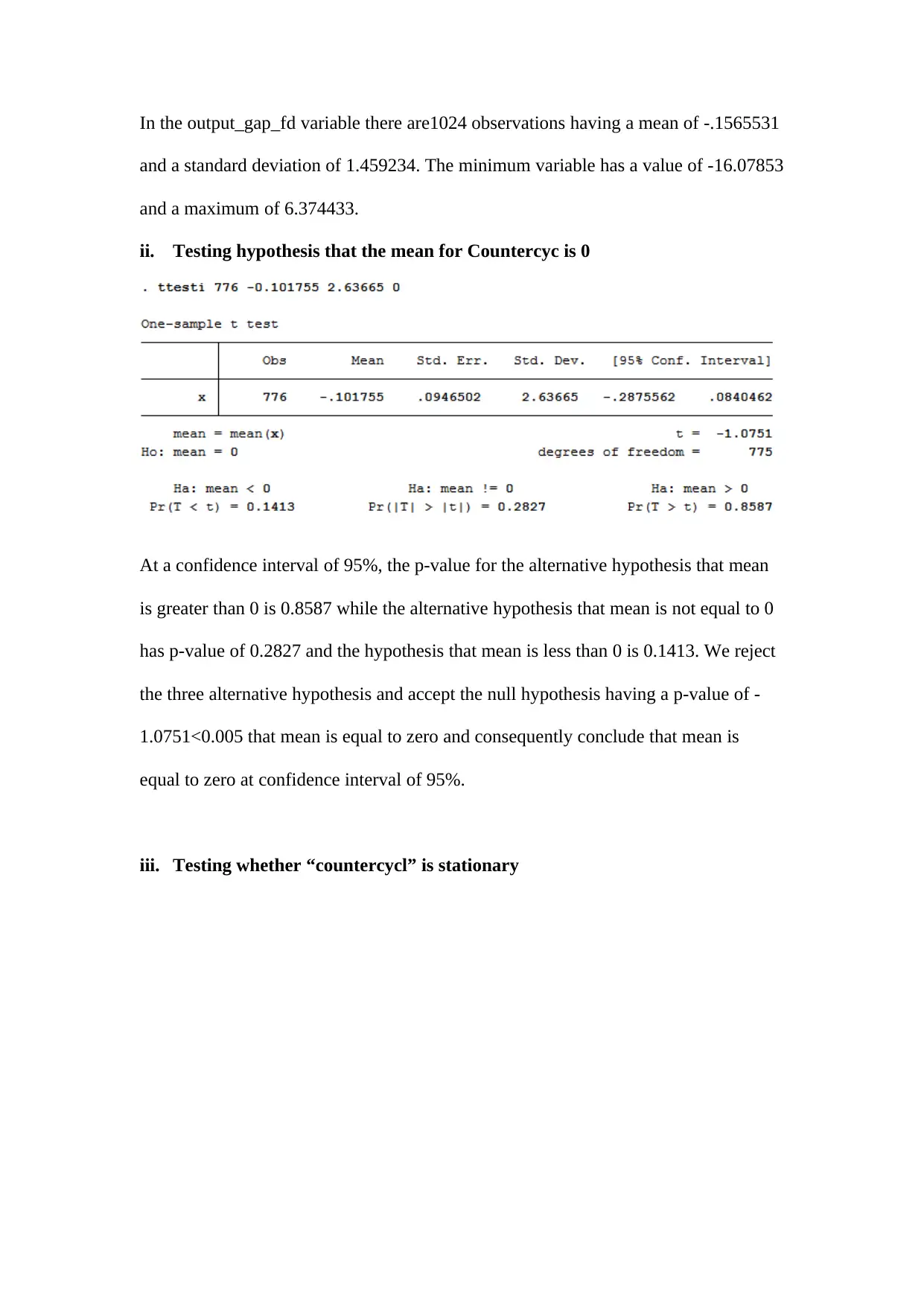
In the output_gap_fd variable there are1024 observations having a mean of -.1565531
and a standard deviation of 1.459234. The minimum variable has a value of -16.07853
and a maximum of 6.374433.
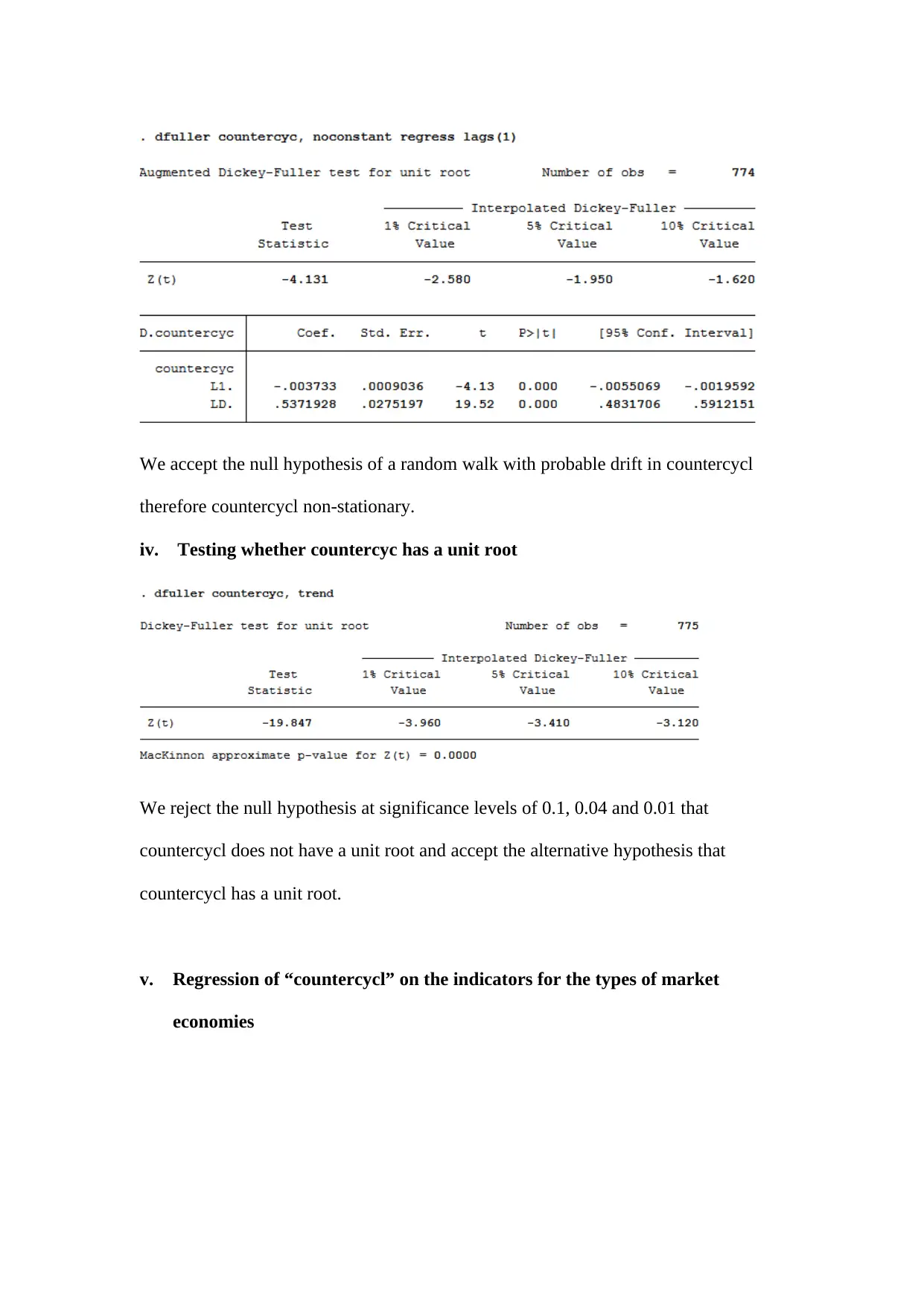
ii. Testing hypothesis that the mean for Countercyc is 0
At a confidence interval of 95%, the p-value for the alternative hypothesis that mean
is greater than 0 is 0.8587 while the alternative hypothesis that mean is not equal to 0
has p-value of 0.2827 and the hypothesis that mean is less than 0 is 0.1413. We reject
the three alternative hypothesis and accept the null hypothesis having a p-value of -
1.0751<0.005 that mean is equal to zero and consequently conclude that mean is
equal to zero at confidence interval of 95%.
iii. Testing whether “countercycl” is stationary
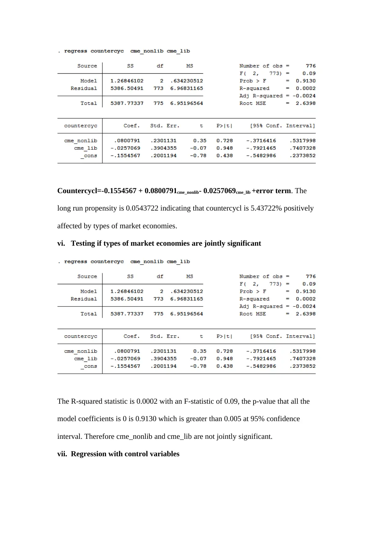
We accept the null hypothesis of a random walk with probable drift in countercycl
therefore countercycl non-stationary.
iv. Testing whether countercyc has a unit root
We reject the null hypothesis at significance levels of 0.1, 0.04 and 0.01 that
countercycl does not have a unit root and accept the alternative hypothesis that
countercycl has a unit root.
v. Regression of “countercycl” on the indicators for the types of market
economies
⊘ This is a preview!⊘
Do you want full access?
Subscribe today to unlock all pages.

Trusted by 1+ million students worldwide
Countercycl=-0.1554567 + 0.0800791cme_nonlib- 0.0257069cme_lib +error term. The
long run propensity is 0.0543722 indicating that countercycl is 5.43722% positively
affected by types of market economies.
vi. Testing if types of market economies are jointly significant
The R-squared statistic is 0.0002 with an F-statistic of 0.09, the p-value that all the
model coefficients is 0 is 0.9130 which is greater than 0.005 at 95% confidence
interval. Therefore cme_nonlib and cme_lib are not jointly significant.
vii. Regression with control variables
Paraphrase This Document
Need a fresh take? Get an instant paraphrase of this document with our AI Paraphraser
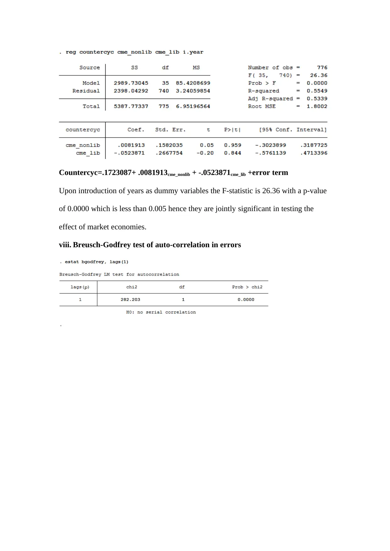
Countercyc=.1723087+ .0081913cme_nonlib + -.0523871cme_lib +error term
Upon introduction of years as dummy variables the F-statistic is 26.36 with a p-value
of 0.0000 which is less than 0.005 hence they are jointly significant in testing the
effect of market economies.
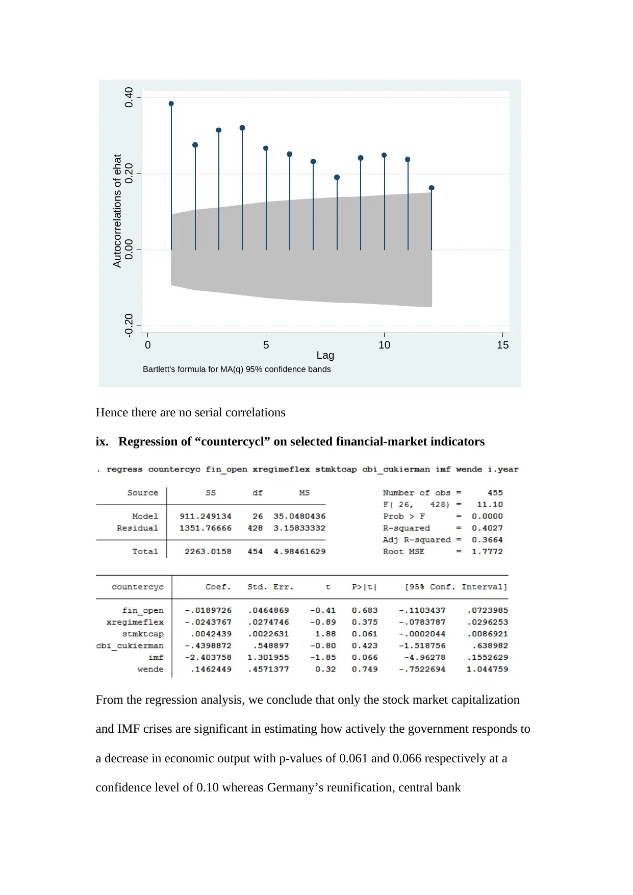
viii. Breusch-Godfrey test of auto-correlation in errors
Upon introduction of years as dummy variables the F-statistic is 26.36 with a p-value
of 0.0000 which is less than 0.005 hence they are jointly significant in testing the
effect of market economies.
viii. Breusch-Godfrey test of auto-correlation in errors
-0.20 0.00 0.20 0.40
Autocorrelations of ehat
0 5 10 15
Lag
Bartlett's formula for MA(q) 95% confidence bands
Hence there are no serial correlations
ix. Regression of “countercycl” on selected financial-market indicators
From the regression analysis, we conclude that only the stock market capitalization
and IMF crises are significant in estimating how actively the government responds to
a decrease in economic output with p-values of 0.061 and 0.066 respectively at a
confidence level of 0.10 whereas Germany’s reunification, central bank
⊘ This is a preview!⊘
Do you want full access?
Subscribe today to unlock all pages.

Trusted by 1+ million students worldwide
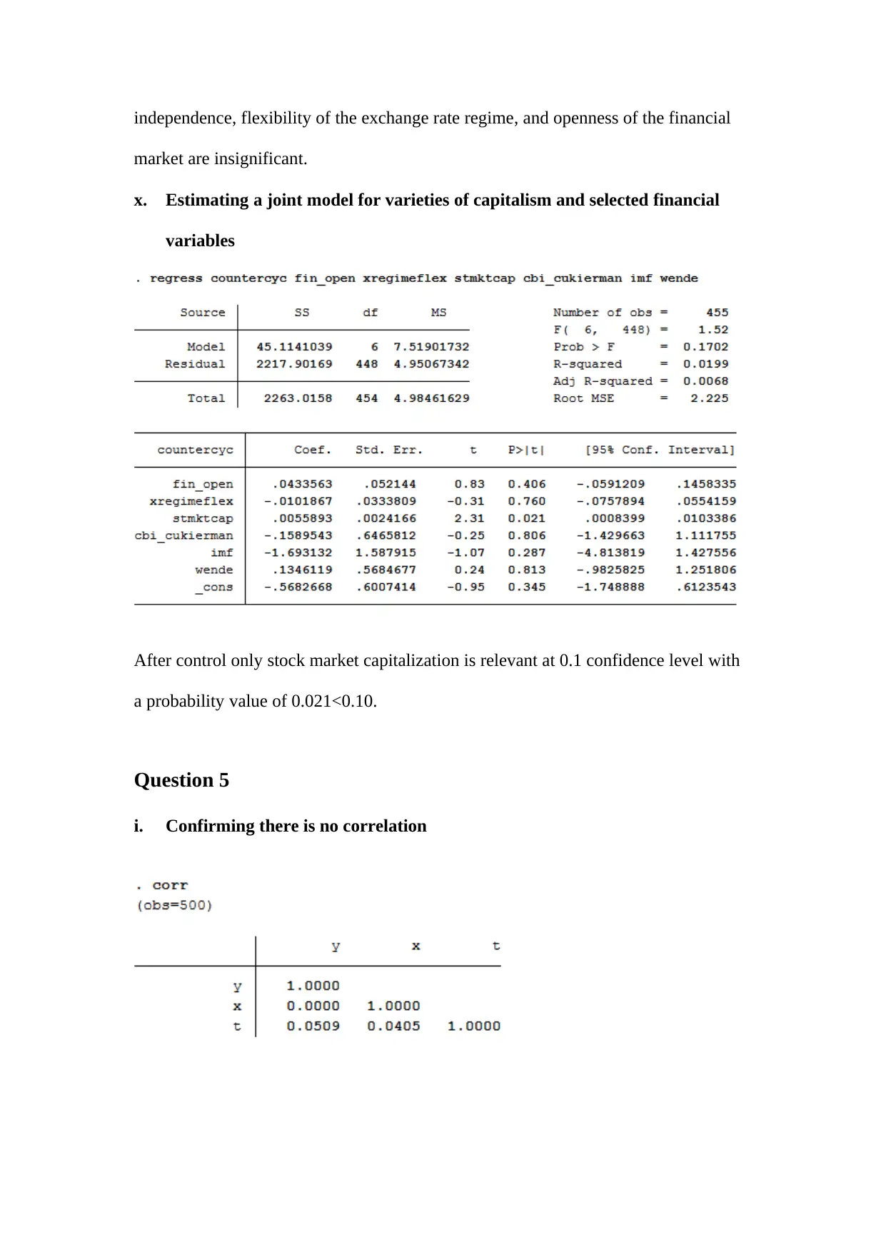
independence, flexibility of the exchange rate regime, and openness of the financial
market are insignificant.
x. Estimating a joint model for varieties of capitalism and selected financial
variables
After control only stock market capitalization is relevant at 0.1 confidence level with
a probability value of 0.021<0.10.
Question 5
i. Confirming there is no correlation
market are insignificant.
x. Estimating a joint model for varieties of capitalism and selected financial
variables
After control only stock market capitalization is relevant at 0.1 confidence level with
a probability value of 0.021<0.10.
Question 5
i. Confirming there is no correlation
Paraphrase This Document
Need a fresh take? Get an instant paraphrase of this document with our AI Paraphraser
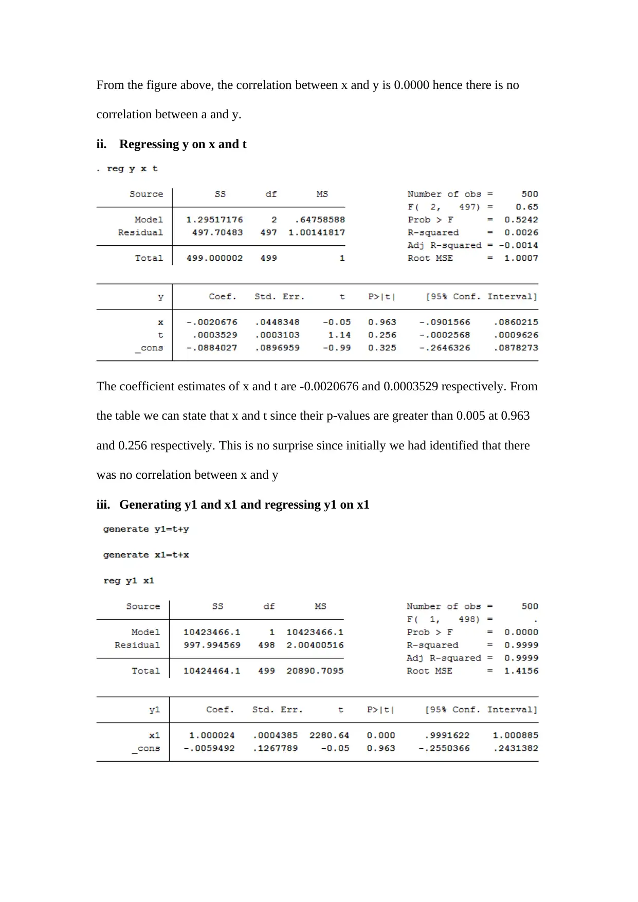
From the figure above, the correlation between x and y is 0.0000 hence there is no
correlation between a and y.
ii. Regressing y on x and t
The coefficient estimates of x and t are -0.0020676 and 0.0003529 respectively. From
the table we can state that x and t since their p-values are greater than 0.005 at 0.963
and 0.256 respectively. This is no surprise since initially we had identified that there
was no correlation between x and y
iii. Generating y1 and x1 and regressing y1 on x1
The coefficient x1 has a coefficient estimate of 1.0000024 and hence is significant.
(Deborah, 2018) argues that an estimate of more than +.30 indicates a strong
relationship and hence significant in estimating target variable. In our case the +1
coefficient estimate indicates a strong relationship. Additionally the p-value for x1 is
0.000 which is less than 0.005 hence significant.
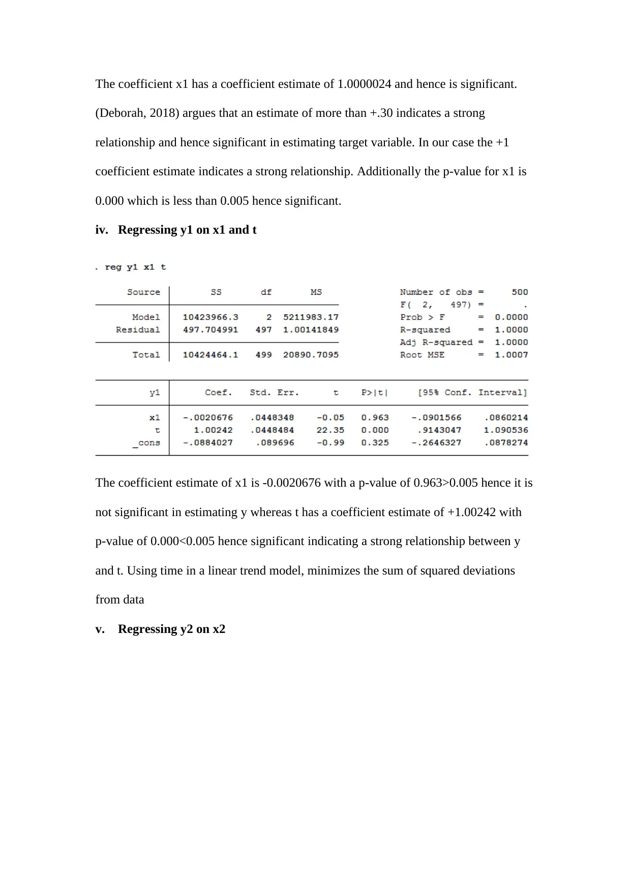
iv. Regressing y1 on x1 and t
The coefficient estimate of x1 is -0.0020676 with a p-value of 0.963>0.005 hence it is
not significant in estimating y whereas t has a coefficient estimate of +1.00242 with
p-value of 0.000<0.005 hence significant indicating a strong relationship between y
and t. Using time in a linear trend model, minimizes the sum of squared deviations
from data
v. Regressing y2 on x2
⊘ This is a preview!⊘
Do you want full access?
Subscribe today to unlock all pages.

Trusted by 1+ million students worldwide
1 out of 16
Your All-in-One AI-Powered Toolkit for Academic Success.
+13062052269
info@desklib.com
Available 24*7 on WhatsApp / Email
![[object Object]](/_next/static/media/star-bottom.7253800d.svg)
Unlock your academic potential
Copyright © 2020–2026 A2Z Services. All Rights Reserved. Developed and managed by ZUCOL.
