Financial Econometrics: Regression Modeling of Greece's Economy Data

This report delves into the application of financial econometrics to analyze the Greek economy, focusing on national income and inflation rates. It employs regression models and various tests, including Durbin-Watson (DW), Lagrange Multiplier (LM), and Ramsey RESET, to assess autocorrelation, specification errors, and heteroscedasticity. The report evaluates regression results using economic, statistical, and econometric criteria, suggesting improvements through data transformation and polynomial regression. It further discusses specific-to-general (S-G) and general-to-specific approaches in time series regression, addressing spurious regression. Finally, it explores the differences between conditional and unconditional variances and the application of ARCH and GARCH models, particularly in the context of bond returns. Desklib provides access to similar solved assignments and past papers for students.

FINANCIAL
ECONOMETRICS

TABLE OF CONTENTS
INTRODUCTION...........................................................................................................................4
QUESTION 1..................................................................................................................................4
1. Testing for autocorrelation by using Durbin-Watson (DW) and Lagrange Multiplier (LM)
tests..............................................................................................................................................5
2. Testing specification errors by using Ramsey Regression Equation Specification Error Test
(RESET)......................................................................................................................................7
3. Test for heteroscedasticity.......................................................................................................8
4. Evaluating regression results through using economic, statistical and econometric criteria...9
 10
5. Explaining the manner in which regression results can be improved...................................10
QUESTION 2................................................................................................................................11
Presenting the attractiveness of specific-to-general (S-G) and general-to-specific approaches
related to time series regression models....................................................................................11
QUESTION 3................................................................................................................................11
i. Explaining the difference between the conditional variance and unconditional variance of r
...................................................................................................................................................11
ii. Outlining ARCH and GARCH models that helps in resolving problems.............................12
iii. Assessing the extent to which variance of 𝑒 affects the return on the bond and apply
GARCH model in this regard....................................................................................................12
iv. GARCH model and case.......................................................................................................12
QUESTION 4................................................................................................................................13
(a) Defining below mentioned aspects along with the suitable examples.................................13
i. Covariance Stationary.............................................................................................................13
ii. Trend Stationary....................................................................................................................13

iii. Difference Stationary...........................................................................................................13
(b) Presenting decompositions relevant for trend stationary and stationary processes along
with its usefulness......................................................................................................................14
CONCLUSION..............................................................................................................................14
REFERENCES..............................................................................................................................15
...................................................................................................................................................15

INTRODUCTION
Econometrics implies for the application of statistical and mathematical theories
pertaining to economics. Such tool as well as theoretical framework provides high level of
assistance in testing hypothesis and forecasting future trends. Field of econometrics lays high
level of emphasis on undertaking economic models and testing variables through the means of
statistical trial. Econometrics can be distinguished into two types such as theoretical and applied
which helps analyst in resolving specific issue. The present report will provide deeper insight
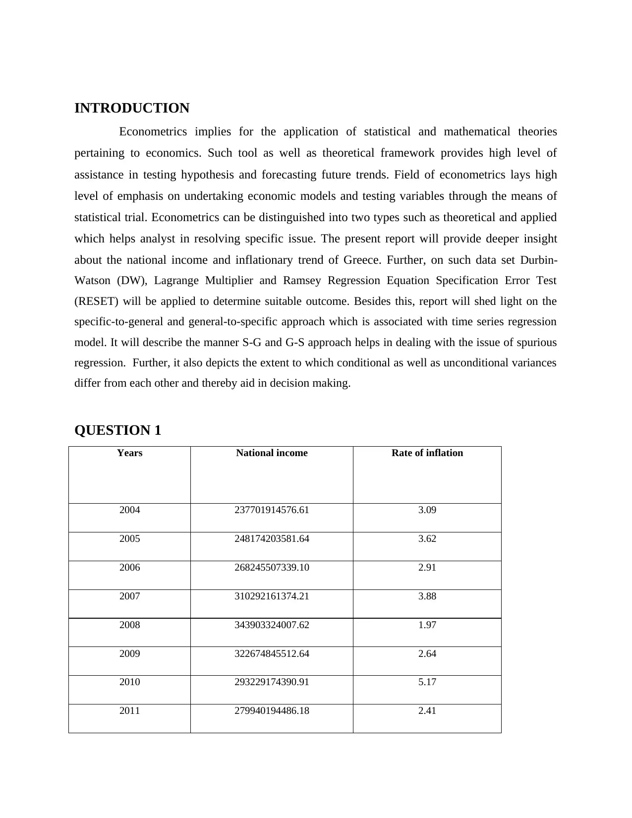
about the national income and inflationary trend of Greece. Further, on such data set Durbin-
Watson (DW), Lagrange Multiplier and Ramsey Regression Equation Specification Error Test
(RESET) will be applied to determine suitable outcome. Besides this, report will shed light on the
specific-to-general and general-to-specific approach which is associated with time series regression
model. It will describe the manner S-G and G-S approach helps in dealing with the issue of spurious
regression. Further, it also depicts the extent to which conditional as well as unconditional variances
differ from each other and thereby aid in decision making.
QUESTION 1
Years National income Rate of inflation
2004 237701914576.61 3.09
2005 248174203581.64 3.62
2006 268245507339.10 2.91
2007 310292161374.21 3.88
2008 343903324007.62 1.97
2009 322674845512.64 2.64
2010 293229174390.91 5.17
2011 279940194486.18 2.41

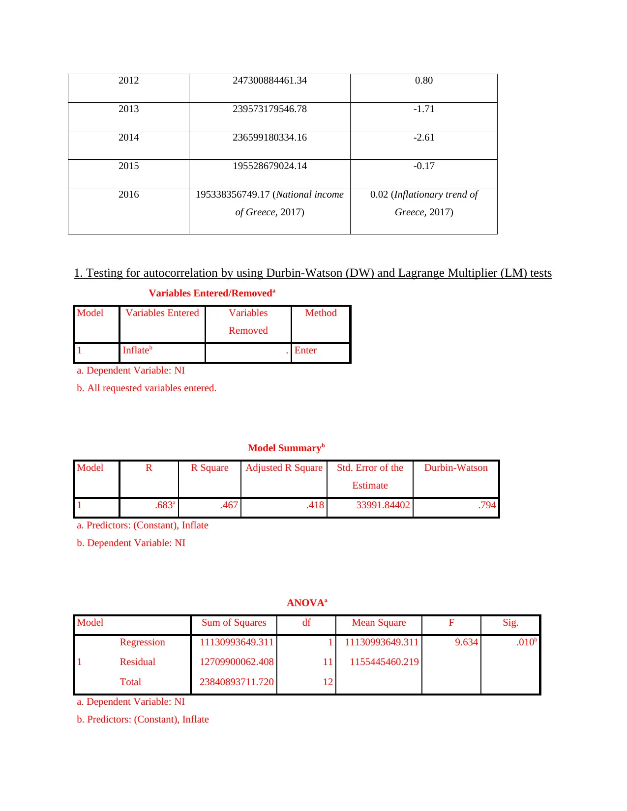
2012 247300884461.34 0.80
2013 239573179546.78 -1.71
2014 236599180334.16 -2.61
2015 195528679024.14 -0.17
2016 195338356749.17 (National income
of Greece, 2017)
0.02 (Inflationary trend of
Greece, 2017)
1. Testing for autocorrelation by using Durbin-Watson (DW) and Lagrange Multiplier (LM) tests
Variables Entered/Removeda
Model Variables Entered Variables
Removed
Method
1 Inflateb . Enter
a. Dependent Variable: NI
b. All requested variables entered.
Model Summaryb
Model R R Square Adjusted R Square Std. Error of the
Estimate
Durbin-Watson
1 .683a .467 .418 33991.84402 .794
a. Predictors: (Constant), Inflate
b. Dependent Variable: NI
ANOVAa
Model Sum of Squares df Mean Square F Sig.
1
Regression 11130993649.311 1 11130993649.311 9.634 .010b
Residual 12709900062.408 11 1155445460.219
Total 23840893711.720 12
a. Dependent Variable: NI
b. Predictors: (Constant), Inflate

Coefficientsa
Model Unstandardized Coefficients Standardized
Coefficients
t Sig.
B Std. Error Beta
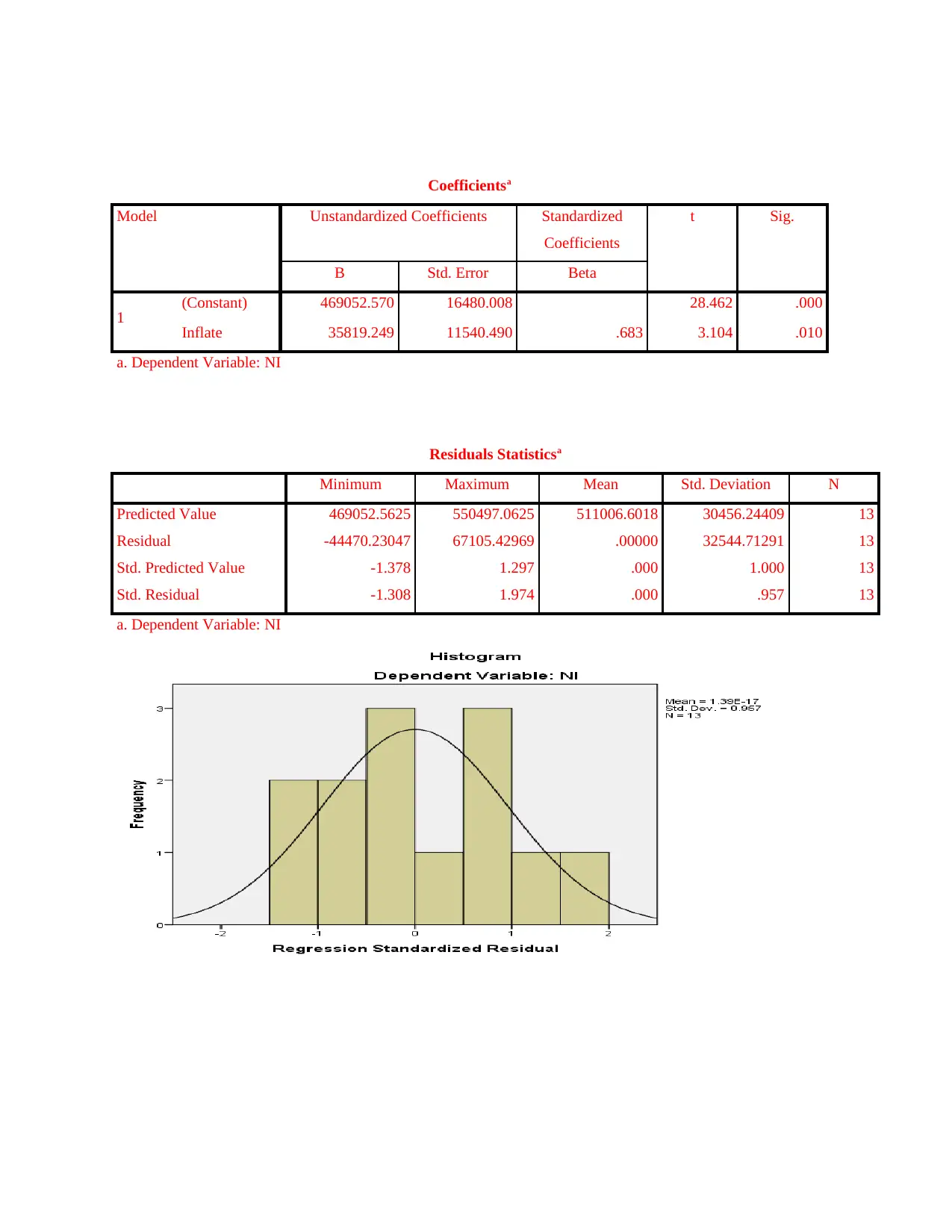
1 (Constant) 469052.570 16480.008 28.462 .000
Inflate 35819.249 11540.490 .683 3.104 .010
a. Dependent Variable: NI
Residuals Statisticsa
Minimum Maximum Mean Std. Deviation N
Predicted Value 469052.5625 550497.0625 511006.6018 30456.24409 13
Residual -44470.23047 67105.42969 .00000 32544.71291 13
Std. Predicted Value -1.378 1.297 .000 1.000 13
Std. Residual -1.308 1.974 .000 .957 13
a. Dependent Variable: NI

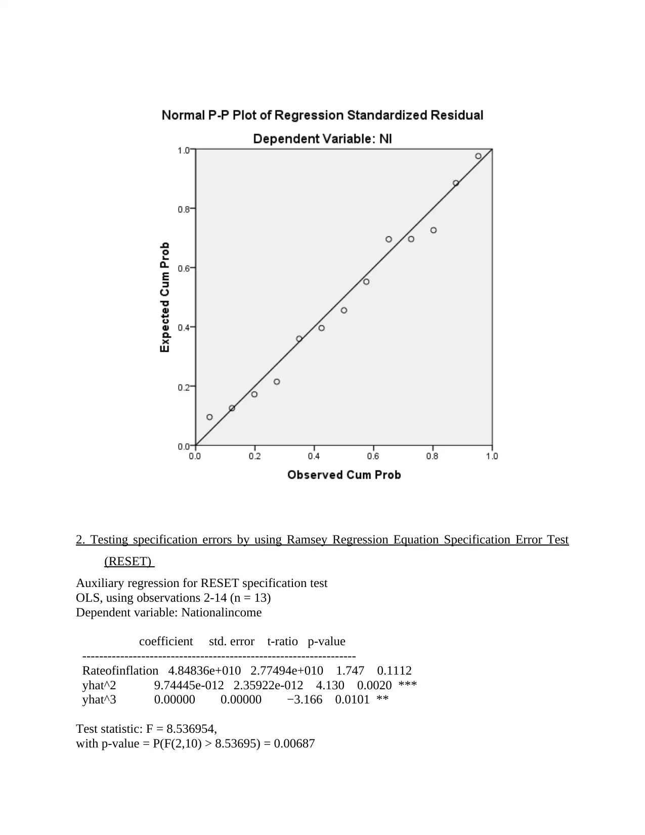
2. Testing specification errors by using Ramsey Regression Equation Specification Error Test
(RESET)
Auxiliary regression for RESET specification test
OLS, using observations 2-14 (n = 13)
Dependent variable: Nationalincome
coefficient std. error t-ratio p-value
-----------------------------------------------------------------
Rateofinflation 4.84836e+010 2.77494e+010 1.747 0.1112
yhat^2 9.74445e-012 2.35922e-012 4.130 0.0020 ***
yhat^3 0.00000 0.00000 −3.166 0.0101 **
Test statistic: F = 8.536954,
with p-value = P(F(2,10) > 8.53695) = 0.00687

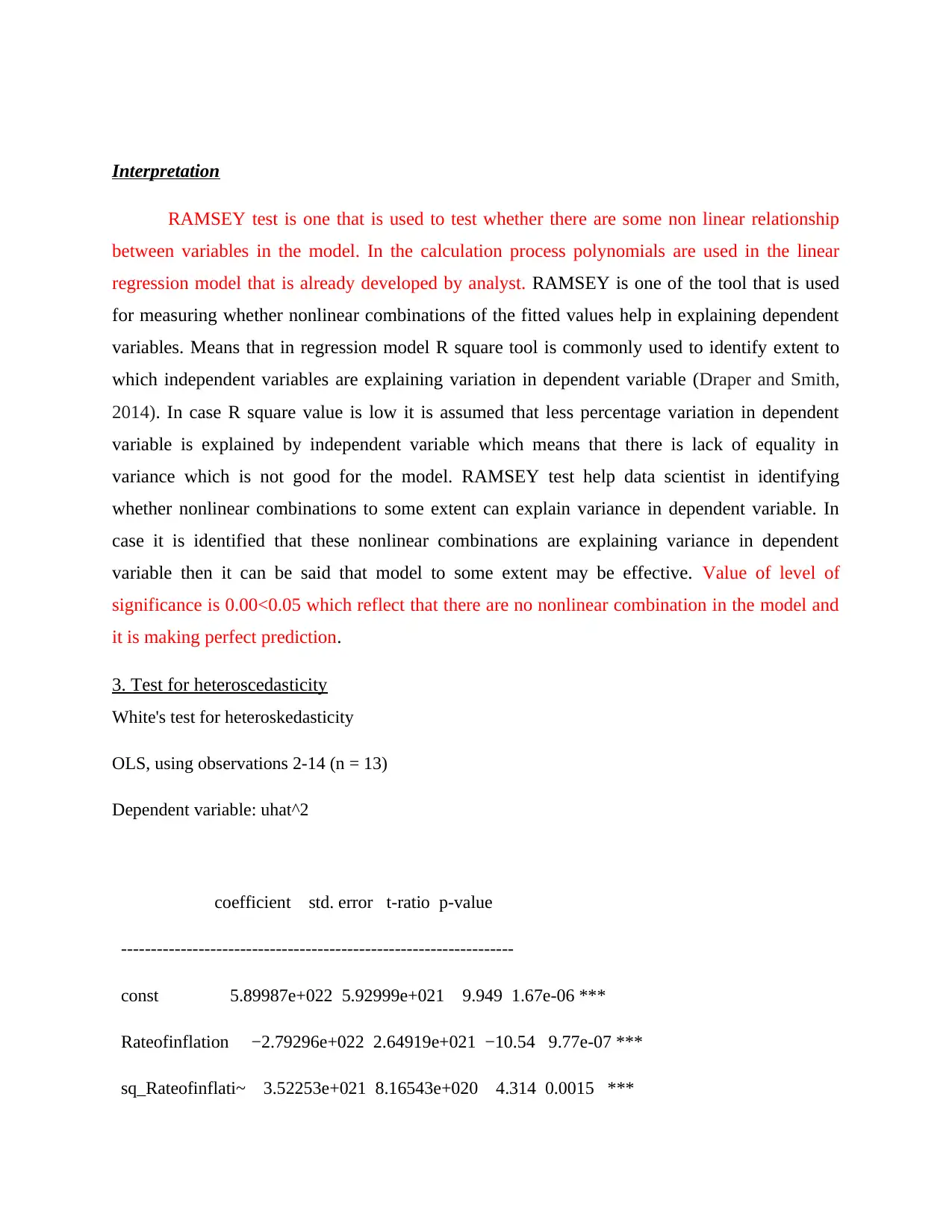
Interpretation
RAMSEY test is one that is used to test whether there are some non linear relationship
between variables in the model. In the calculation process polynomials are used in the linear
regression model that is already developed by analyst. RAMSEY is one of the tool that is used
for measuring whether nonlinear combinations of the fitted values help in explaining dependent
variables. Means that in regression model R square tool is commonly used to identify extent to
which independent variables are explaining variation in dependent variable (Draper and Smith,
2014). In case R square value is low it is assumed that less percentage variation in dependent
variable is explained by independent variable which means that there is lack of equality in
variance which is not good for the model. RAMSEY test help data scientist in identifying
whether nonlinear combinations to some extent can explain variance in dependent variable. In
case it is identified that these nonlinear combinations are explaining variance in dependent
variable then it can be said that model to some extent may be effective. Value of level of
significance is 0.00<0.05 which reflect that there are no nonlinear combination in the model and
it is making perfect prediction.
3. Test for heteroscedasticity
White's test for heteroskedasticity
OLS, using observations 2-14 (n = 13)
Dependent variable: uhat^2
coefficient std. error t-ratio p-value
------------------------------------------------------------------
const 5.89987e+022 5.92999e+021 9.949 1.67e-06 ***
Rateofinflation −2.79296e+022 2.64919e+021 −10.54 9.77e-07 ***
sq_Rateofinflati~ 3.52253e+021 8.16543e+020 4.314 0.0015 ***

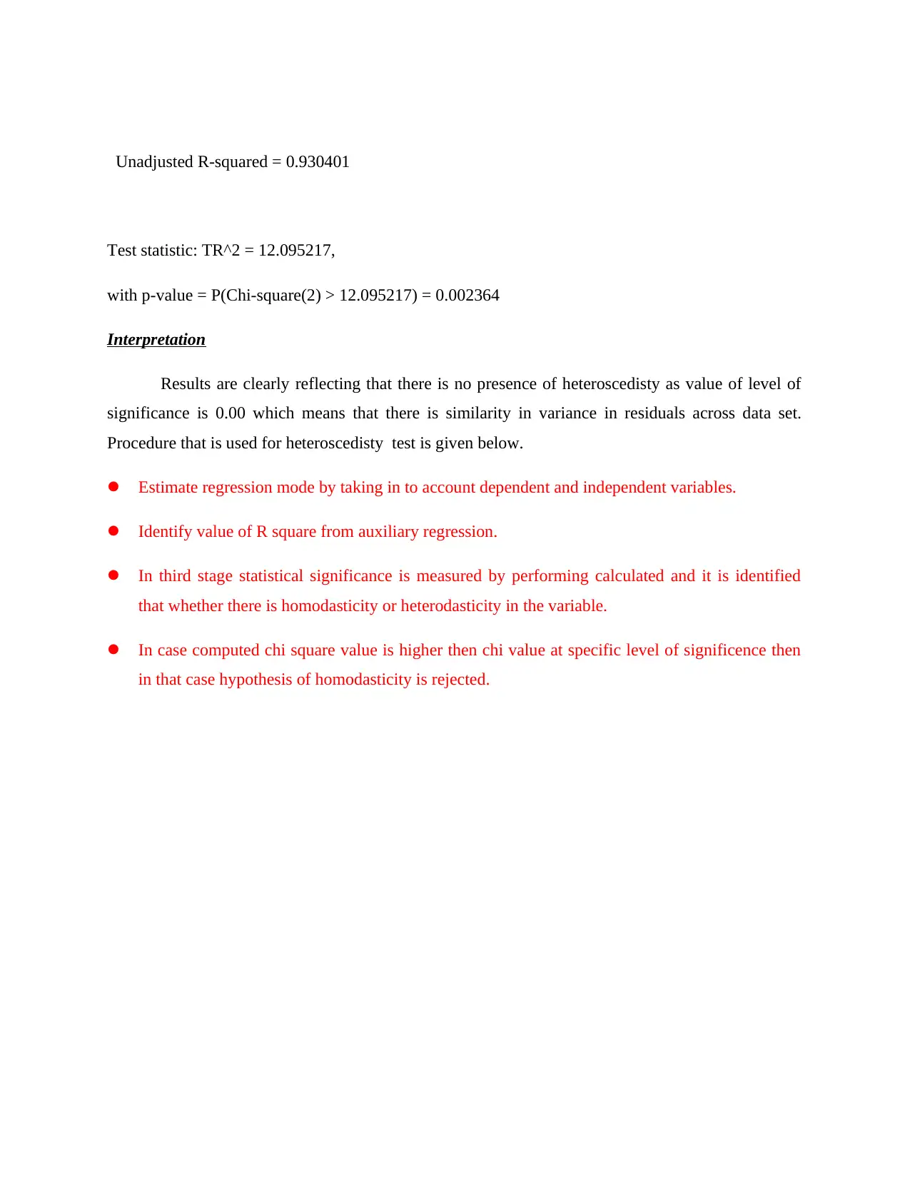
Unadjusted R-squared = 0.930401
Test statistic: TR^2 = 12.095217,
with p-value = P(Chi-square(2) > 12.095217) = 0.002364
Interpretation
Results are clearly reflecting that there is no presence of heteroscedisty as value of level of
significance is 0.00 which means that there is similarity in variance in residuals across data set.
Procedure that is used for heteroscedisty test is given below.
 Estimate regression mode by taking in to account dependent and independent variables.
 Identify value of R square from auxiliary regression.
 In third stage statistical significance is measured by performing calculated and it is identified
that whether there is homodasticity or heterodasticity in the variable.
 In case computed chi square value is higher then chi value at specific level of significence then
in that case hypothesis of homodasticity is rejected.

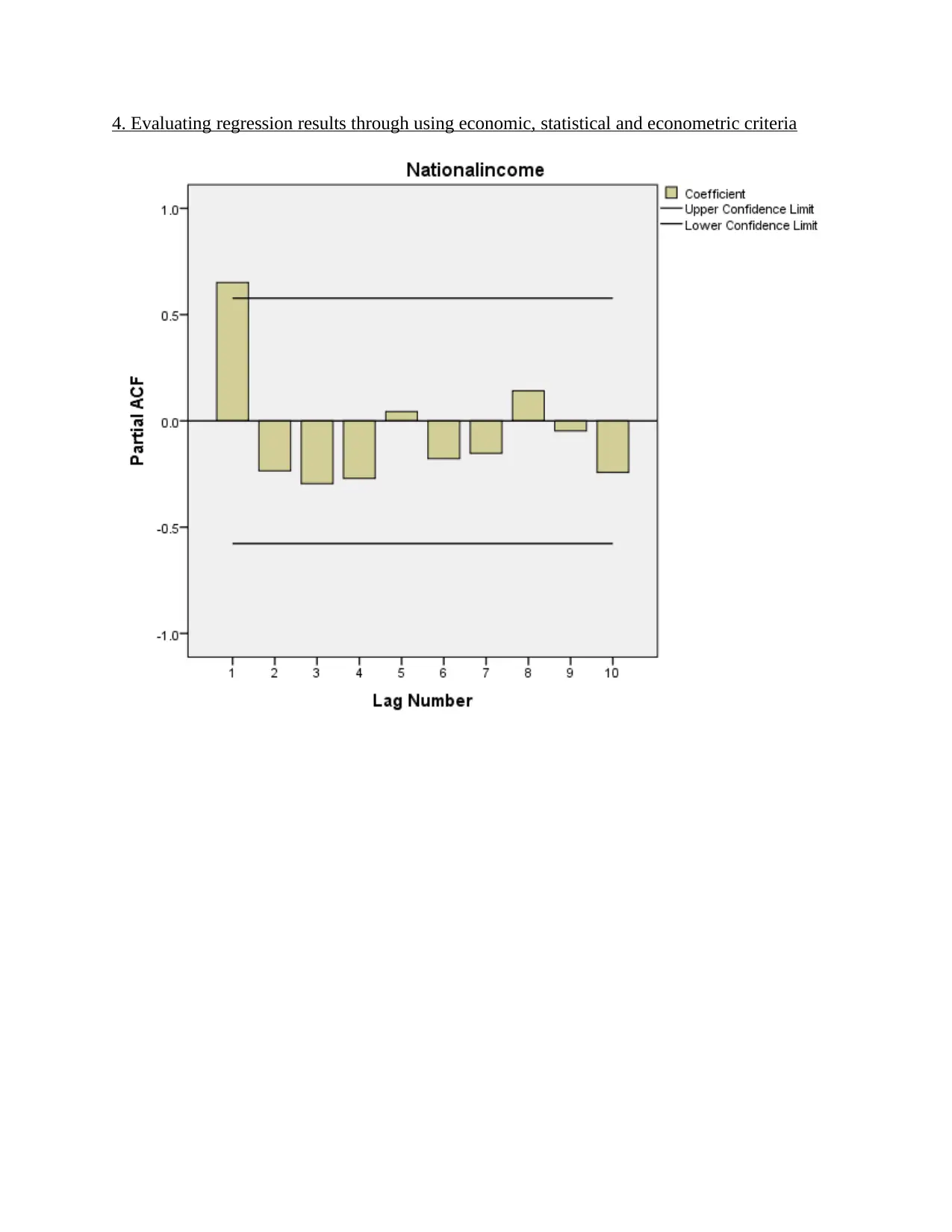
4. Evaluating regression results through using economic, statistical and econometric criteria

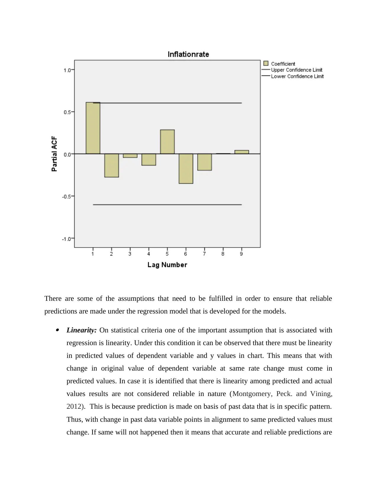
There are some of the assumptions that need to be fulfilled in order to ensure that reliable
predictions are made under the regression model that is developed for the models.
 Linearity: On statistical criteria one of the important assumption that is associated with
regression is linearity. Under this condition it can be observed that there must be linearity
in predicted values of dependent variable and y values in chart. This means that with
change in original value of dependent variable at same rate change must come in
predicted values. In case it is identified that there is linearity among predicted and actual
values results are not considered reliable in nature (Montgomery, Peck. and Vining,
2012). This is because prediction is made on basis of past data that is in specific pattern.
Thus, with change in past data variable points in alignment to same predicted values must
change. If same will not happened then it means that accurate and reliable predictions are

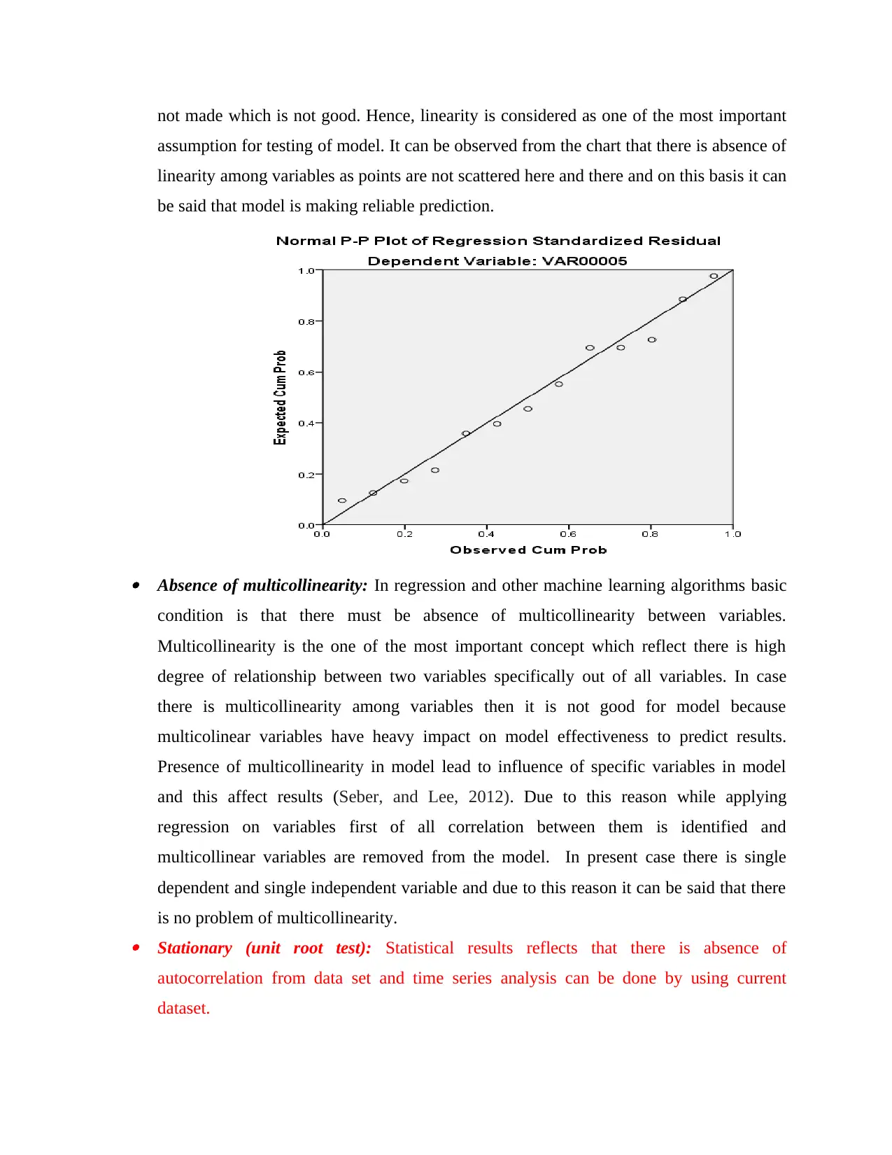
not made which is not good. Hence, linearity is considered as one of the most important
assumption for testing of model. It can be observed from the chart that there is absence of
linearity among variables as points are not scattered here and there and on this basis it can
be said that model is making reliable prediction.
 Absence of multicollinearity: In regression and other machine learning algorithms basic
condition is that there must be absence of multicollinearity between variables.
Multicollinearity is the one of the most important concept which reflect there is high
degree of relationship between two variables specifically out of all variables. In case
there is multicollinearity among variables then it is not good for model because
multicolinear variables have heavy impact on model effectiveness to predict results.
Presence of multicollinearity in model lead to influence of specific variables in model
and this affect results (Seber, and Lee, 2012). Due to this reason while applying
regression on variables first of all correlation between them is identified and
multicollinear variables are removed from the model. In present case there is single
dependent and single independent variable and due to this reason it can be said that there
is no problem of multicollinearity. Stationary (unit root test): Statistical results reflects that there is absence of
autocorrelation from data set and time series analysis can be done by using current
dataset.