Statistical Regression Analysis and Diagnostics Report 2020

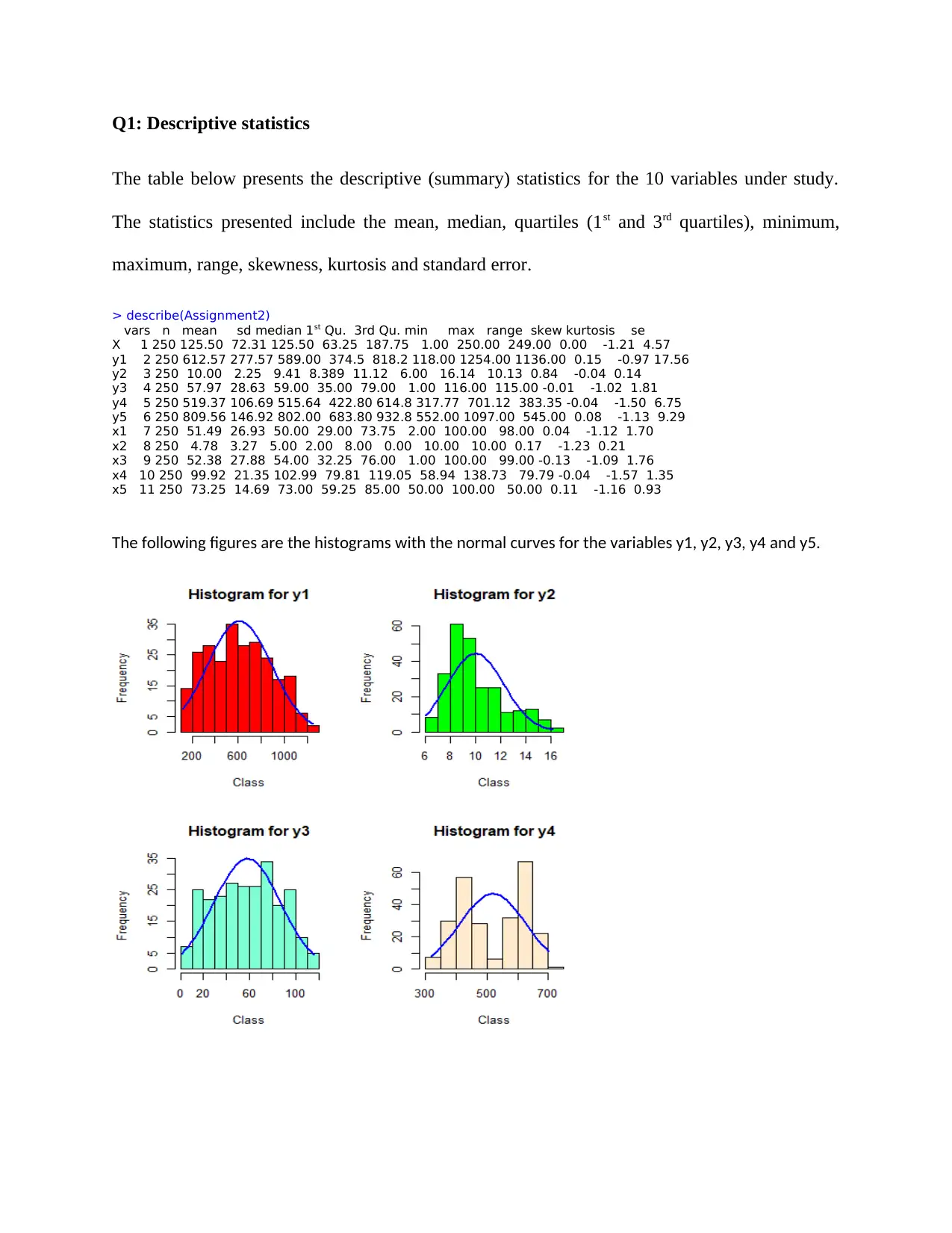
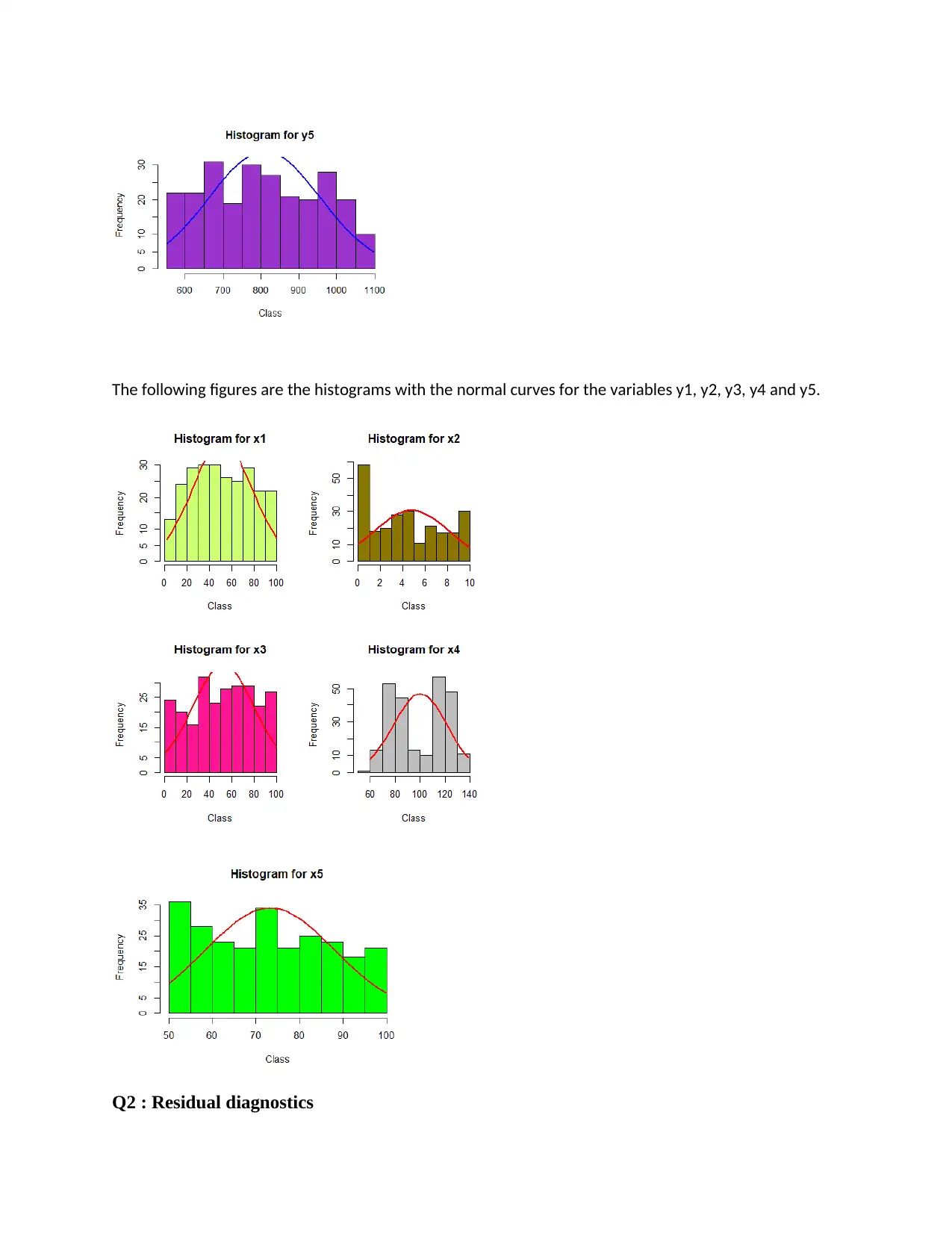
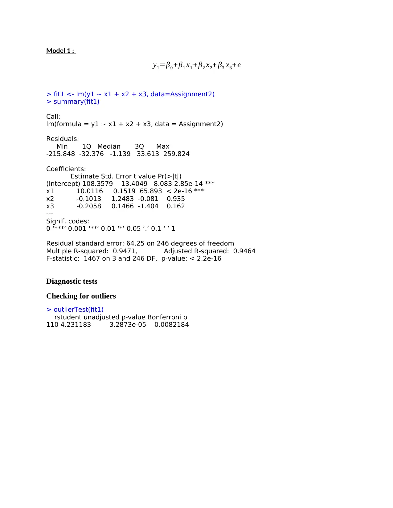
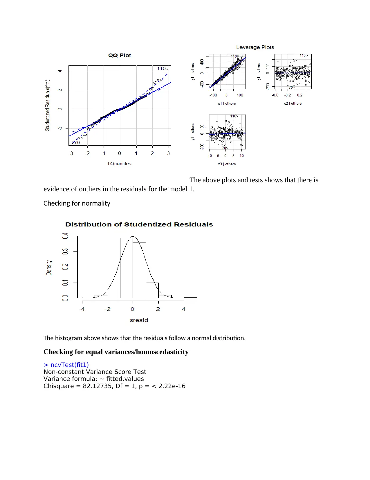
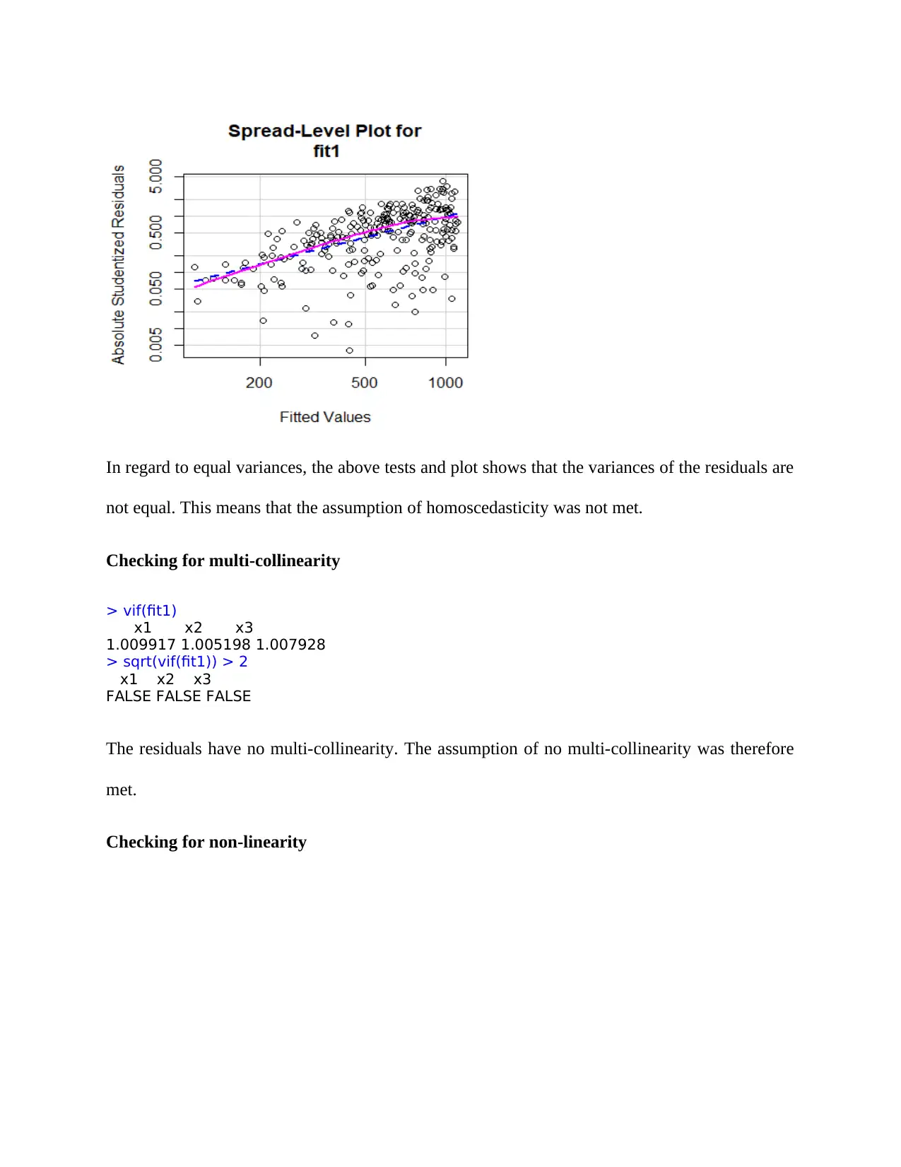
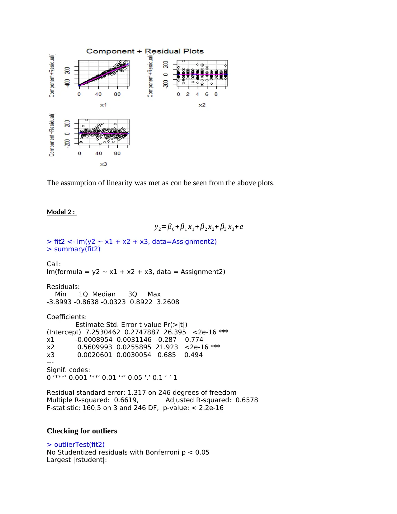
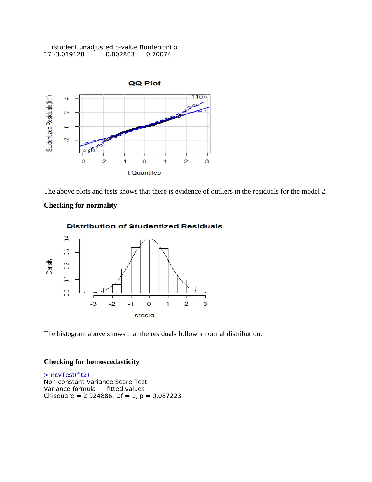
This assignment solution provides a comprehensive analysis of regression models and residual diagnostics. It begins with descriptive statistics for ten variables, including mean, median, quartiles, and skewness. The solution then assesses five regression models (fit1 to fit5), checking for outliers, normality, homoscedasticity, multicollinearity, and linearity. Diagnostic tests such as outlierTest, ncvTest, and vif are used to validate model assumptions. Additionally, the assignment includes an analysis of the 'prestige' dataset, creating scatter plot matrices and descriptive statistics. Finally, distinct simple regression models are built to predict prestige based on education, income and gender, evaluating their significance and R-squared values. The analysis uses statistical tools and tests to ensure the robustness and validity of the regression models.

UNIVARIATE ANALYSIS II: REGRESSION
Student Name:
Instructor Name:
Course Number:
20th February 2020

Q1: Descriptive statistics
The table below presents the descriptive (summary) statistics for the 10 variables under study.
The statistics presented include the mean, median, quartiles (1st and 3rd quartiles), minimum,
maximum, range, skewness, kurtosis and standard error.
> describe(Assignment2)
vars n mean sd median 1st Qu. 3rd Qu. min max range skew kurtosis se
X 1 250 125.50 72.31 125.50 63.25 187.75 1.00 250.00 249.00 0.00 -1.21 4.57
y1 2 250 612.57 277.57 589.00 374.5 818.2 118.00 1254.00 1136.00 0.15 -0.97 17.56
y2 3 250 10.00 2.25 9.41 8.389 11.12 6.00 16.14 10.13 0.84 -0.04 0.14
y3 4 250 57.97 28.63 59.00 35.00 79.00 1.00 116.00 115.00 -0.01 -1.02 1.81
y4 5 250 519.37 106.69 515.64 422.80 614.8 317.77 701.12 383.35 -0.04 -1.50 6.75
y5 6 250 809.56 146.92 802.00 683.80 932.8 552.00 1097.00 545.00 0.08 -1.13 9.29
x1 7 250 51.49 26.93 50.00 29.00 73.75 2.00 100.00 98.00 0.04 -1.12 1.70
x2 8 250 4.78 3.27 5.00 2.00 8.00 0.00 10.00 10.00 0.17 -1.23 0.21
x3 9 250 52.38 27.88 54.00 32.25 76.00 1.00 100.00 99.00 -0.13 -1.09 1.76
x4 10 250 99.92 21.35 102.99 79.81 119.05 58.94 138.73 79.79 -0.04 -1.57 1.35
x5 11 250 73.25 14.69 73.00 59.25 85.00 50.00 100.00 50.00 0.11 -1.16 0.93
The following figures are the histograms with the normal curves for the variables y1, y2, y3, y4 and y5.

The following figures are the histograms with the normal curves for the variables y1, y2, y3, y4 and y5.
Q2 : Residual diagnostics

Model 1 :
y1=β0 + β1 x1 + β2 x2+ β3 x3+ e
> fit1 <- lm(y1 ~ x1 + x2 + x3, data=Assignment2)
> summary(fit1)
Call:
lm(formula = y1 ~ x1 + x2 + x3, data = Assignment2)
Residuals:
Min 1Q Median 3Q Max
-215.848 -32.376 -1.139 33.613 259.824
Coefficients:
Estimate Std. Error t value Pr(>|t|)
(Intercept) 108.3579 13.4049 8.083 2.85e-14 ***
x1 10.0116 0.1519 65.893 < 2e-16 ***
x2 -0.1013 1.2483 -0.081 0.935
x3 -0.2058 0.1466 -1.404 0.162
---
Signif. codes:
0 ‘***’ 0.001 ‘**’ 0.01 ‘*’ 0.05 ‘.’ 0.1 ‘ ’ 1
Residual standard error: 64.25 on 246 degrees of freedom
Multiple R-squared: 0.9471, Adjusted R-squared: 0.9464
F-statistic: 1467 on 3 and 246 DF, p-value: < 2.2e-16
Diagnostic tests
Checking for outliers
> outlierTest(fit1)
rstudent unadjusted p-value Bonferroni p
110 4.231183 3.2873e-05 0.0082184

The above plots and tests shows that there is
evidence of outliers in the residuals for the model 1.
Checking for normality
The histogram above shows that the residuals follow a normal distribution.
Checking for equal variances/homoscedasticity
> ncvTest(fit1)
Non-constant Variance Score Test
Variance formula: ~ fitted.values
Chisquare = 82.12735, Df = 1, p = < 2.22e-16

In regard to equal variances, the above tests and plot shows that the variances of the residuals are
not equal. This means that the assumption of homoscedasticity was not met.
Checking for multi-collinearity
> vif(fit1)
x1 x2 x3
1.009917 1.005198 1.007928
> sqrt(vif(fit1)) > 2
x1 x2 x3
FALSE FALSE FALSE
The residuals have no multi-collinearity. The assumption of no multi-collinearity was therefore
met.
Checking for non-linearity

The assumption of linearity was met as con be seen from the above plots.
Model 2 :
y2=β0 + β1 x1 + β2 x2+ β3 x3+ e
> fit2 <- lm(y2 ~ x1 + x2 + x3, data=Assignment2)
> summary(fit2)
Call:
lm(formula = y2 ~ x1 + x2 + x3, data = Assignment2)
Residuals:
Min 1Q Median 3Q Max
-3.8993 -0.8638 -0.0323 0.8922 3.2608
Coefficients:
Estimate Std. Error t value Pr(>|t|)
(Intercept) 7.2530462 0.2747887 26.395 <2e-16 ***
x1 -0.0008954 0.0031146 -0.287 0.774
x2 0.5609993 0.0255895 21.923 <2e-16 ***
x3 0.0020601 0.0030054 0.685 0.494
---
Signif. codes:
0 ‘***’ 0.001 ‘**’ 0.01 ‘*’ 0.05 ‘.’ 0.1 ‘ ’ 1
Residual standard error: 1.317 on 246 degrees of freedom
Multiple R-squared: 0.6619, Adjusted R-squared: 0.6578
F-statistic: 160.5 on 3 and 246 DF, p-value: < 2.2e-16
Checking for outliers
> outlierTest(fit2)
No Studentized residuals with Bonferroni p < 0.05
Largest |rstudent|:

rstudent unadjusted p-value Bonferroni p
17 -3.019128 0.002803 0.70074
The above plots and tests shows that there is evidence of outliers in the residuals for the model 2.
Checking for normality
The histogram above shows that the residuals follow a normal distribution.
Checking for homoscedasticity
> ncvTest(fit2)
Non-constant Variance Score Test
Variance formula: ~ fitted.values
Chisquare = 2.924886, Df = 1, p = 0.087223

In regard to equal variances, the above tests and plot shows that the variances of the residuals are
equal. This means that the assumption of homoscedasticity was met.
Checking for multi-collinearity
> vif(fit2)
x1 x2 x3
1.009917 1.005198 1.007928
> sqrt(vif(fit2)) > 2
x1 x2 x3
FALSE FALSE FALSE
The residuals have no multi-collinearity. The assumption of no multi-collinearity was therefore
met.
Checking for non-linearity

The above plots shows that assumption of
linearity was met for model 2.
Model 3 :
y1=β0 + β1 x1 + β2 x2+ β3 x3+ e
> fit3 <- lm(y3 ~ x1 + x2 + x3, data=Assignment2)
> summary(fit3)
Call:
lm(formula = y3 ~ x1 + x2 + x3, data = Assignment2)
Residuals:
Min 1Q Median 3Q Max
-6.189 -3.876 -1.725 2.011 30.512
Coefficients:
Estimate Std. Error t value Pr(>|t|)
(Intercept) 5.81133 1.17643 4.940 1.45e-06 ***
x1 -0.01432 0.01333 -1.074 0.284
x2 0.04400 0.10955 0.402 0.688
x3 1.00579 0.01287 78.170 < 2e-16 ***
---
Signif. codes:
0 ‘***’ 0.001 ‘**’ 0.01 ‘*’ 0.05 ‘.’ 0.1 ‘ ’ 1
Residual standard error: 5.639 on 246 degrees of freedom
Multiple R-squared: 0.9617, Adjusted R-squared: 0.9612
F-statistic: 2057 on 3 and 246 DF, p-value: < 2.2e-16

Checking for outliers
> outlierTest(fit3)
rstudent unadjusted p-value Bonferroni p
161 5.798028 2.0584e-08 5.1461e-06
8 4.262756 2.8832e-05 7.2081e-03
189 3.966351 9.5859e-05 2.3965e-02
The above plots and tests shows that there is evidence of outliers in the residuals for the model 3.
Checking for normality
The normality check showed that the residuals are heavily skewed (right skewed).
Checking for homoscedasticity
> ncvTest(fit3)
Non-constant Variance Score Test
Variance formula: ~ fitted.values
Chisquare = 1.626533, Df = 1, p = 0.20218

From the above results, it is evident that the residuals have equal variances hence assumption of
equal variances was met.
Checking for multi-collinearity
> vif(fit3)
x1 x2 x3
1.009917 1.005198 1.007928
> sqrt(vif(fit3)) > 2
x1 x2 x3
FALSE FALSE FALSE
Results showed that there is no evidence of multi-collinearity for the residuals.
Checking for linearity