Regression Analysis of Cereal Demand: Price, Income, and Consumption

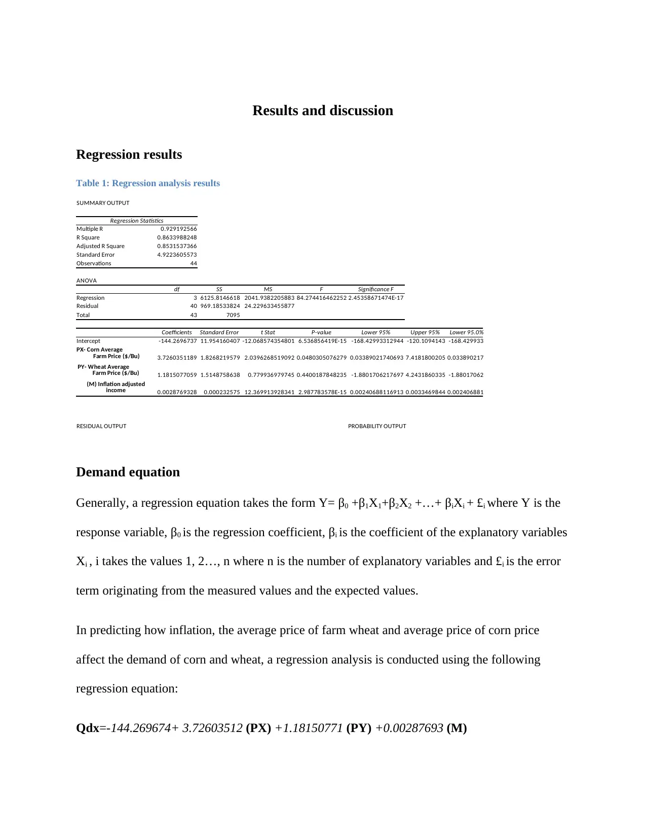
This report presents a regression analysis of cereal demand, focusing on the impact of factors such as corn and wheat prices, as well as inflation-adjusted household income in the U.S. The regression equation Qdx = -144.269674 + 3.72603512(PX) + 1.18150771(PY) + 0.00287693(M) is used to model the relationship, where Qdx represents demand, PX is the average farm price of corn, PY is the average farm price of wheat, and M is the inflation-adjusted income. The results indicate a positive relationship between cereal prices and demand, with a $1,000 increase in corn price leading to a $3.73 increase in demand and a similar increase in wheat price resulting in a $1.18 increase in demand. Inflation-adjusted income has a marginal effect, with a $1,000 increase leading to only a $0.0029 increase in demand. The R-squared value of 0.8633 suggests that 86.33% of the variability in the error term is explained by the model, and the adjusted R-squared of 0.85315 indicates a good fit. ANOVA and t-tests confirm the statistical significance of the variables in predicting cereal demand, highlighting the importance of both price and income factors in influencing consumption patterns among American households.

Results and discussion
Regression results
Table 1: Regression analysis results
SUMMARY OUTPUT
Regression Statistics
Multiple R 0.929192566
R Square 0.8633988248
Adjusted R Square 0.8531537366
Standard Error 4.9223605573
Observations 44
ANOVA
df SS MS F Significance F
Regression 3 6125.8146618 2041.9382205883 84.274416462252 2.45358671474E-17
Residual 40 969.18533824 24.229633455877
Total 43 7095
Coefficients Standard Error t Stat P-value Lower 95% Upper 95% Lower 95.0%
Intercept -144.2696737 11.954160407 -12.068574354801 6.536856419E-15 -168.42993312944 -120.1094143 -168.4299331
3.7260351189 1.8268219579 2.0396268519092 0.0480305076279 0.03389021740693 7.4181800205 0.0338902174
1.1815077059 1.5148758638 0.779936979745 0.4400187848235 -1.8801706217697 4.2431860335 -1.880170622
0.0028769328 0.000232575 12.369913928341 2.987783578E-15 0.00240688116913 0.0033469844 0.0024068812
RESIDUAL OUTPUT PROBABILITY OUTPUT
PX- Corn Average
Farm Price ($/Bu)
PY- Wheat Average
Farm Price ($/Bu)
(M) Inflation adjusted
income
Demand equation
Generally, a regression equation takes the form Y= β0 +β1X1+β2X2 +…+ βiXi + £i where Y is the
response variable, β0 is the regression coefficient, βi is the coefficient of the explanatory variables
Xi , i takes the values 1, 2…, n where n is the number of explanatory variables and £i is the error
term originating from the measured values and the expected values.
In predicting how inflation, the average price of farm wheat and average price of corn price
affect the demand of corn and wheat, a regression analysis is conducted using the following
regression equation:
Qdx=-144.269674+ 3.72603512 (PX) +1.18150771 (PY) +0.00287693 (M)

Where:
Qdx is the demand i.e. wheat and corn consumption
PX is the corn average farm price feed
PY is the corn average farm price of wheat
M is the inflation adjusted income of US households
Interpretation of the Regression results
The coefficient of Corn average farm price is 3.72603512, thus there is a positive relationship
between demand and the corn average farm price. Whereby, an increase in the corn average farm
price by 1,000$ would lead to an increase in the demand of consumption by 3.72603512$, and
the consumption demand would increase by 1.18150771 in case the wheat average farm price
would increase by 1,000$. Additionally, the inflation adjusted income for US households have a
very low marginally effects on the demand of cereal feed whereby an increase in 1,000$ in the
inflation adjusted income would lead to only a 0.00287693$ increase in the demand which is
0.28769% increase, all other factors affecting demand held constant in the mentioned cases.
In comparing the joint effect of combined factors, that is corn average farm price and wheat
average farm price, a joint increase of 1,000$ on both factors would lead to a 4.90754283
increase in demand. Therefore, both wheat and corn feeds have a joint demand where an increase
in demand of one leads to an increase in demand of the other.

Verification of significance
R-Squared, Adjusted-R, Multiple R
From the regression results from table 1 above, the R-squared statistic is 0.8633 which indicate
that 86.33% of the variability in the error term of the response variables can be measured by the
model, whereas the adjusted- R square is 0.85315 indicating that at 85.315% the model is a good
fit. The multiple-R statistic is 0.929193 which is close to 1, indicating that there is strong
correlation between the predictor variables
The adjusted R-squared is often used to test for the goodness of fit while the R-squared statistic
tests the significance of all the statistical variables, where an inclusion of many variables tends to
give a higher R-squared statistical value. However, to test whether the model is a good fit we use
the adjusted R-squared in which case the model used in this study indicates that it is a good fit
for regression.
Other significant statistical values are the:
i. Mean Standard error
ii. ANOVA output
iii. Residual plots
Mean Standard Error
The mean standard error from the output is given by 4.9223606, indicating that the true mean lies
at a ±4.9223606 interval of the predicted mean of the demand such that when all the predictor
variables are zero, the mean is (4.9223606-144.2696737)= -139.35 and (-144.2696737-
4.9223606)= -149.1920343

ANOVA
From the ANOVA table, the mean squared regression is 2041.938221 and the mean square due
to errors is 24.22963346, therefore the F-value is given as 84.27441646. In testing the null
hypothesis of the existence of a relationship between the predictor and response variables, the P-
value from the ANOVA table is 0.000 which is less that the significance level of 0.005. We
therefore fail to reject the null hypothesis and conclude that there is a relationship between the
response and explanatory variables.
Significance of coefficients in the model
In testing whether the various variables are significant in predicting change in the response
variable Qdx, we use the T-test.
i. Significance of the average farm price of corn in predicting demand
From the ANOVA table, the standard error of PX is 1.286822 with a t statistic of 2.03626852;
the P-value for the t test for the significance of PX is 0.000 which is less than 0.05 at a ±95%
confidence interval indicating that it is statistically significant in predicting the response variable
Qdx
ii. Significance of the average farm price of wheat
From the ANOVA table, the standard error of PY is 1.514876 with a t statistic of 0.779937, the
P-value for t test of the significance of PX is 0.04803051 which is less than ±0.05 at a
significance level of 0.05, and hence PX is statistically significant in predicting demand.
iii. Significance of inflation adjusted income of US households
From the ANOVA output, the standard error of M is 0.000232575 with a t statistic of
12.36991393. The P-value for t test for the significance of M is 0.000 which is less than 0.005 at

a ±95% confidence level indicating that M is statistically significant in predicting demand in the
regression model.
Following our results from the regression analysis, it is true to infer that demand of cereals
among American households is influenced by factors such as income and the average household
income. As seen from the deductive analysis, an increase in average income slightly influences
an increase in the demand. However, there are different degrees of the effects of predictor
variables on the response variables where average price of both cereals influence demand more
than the effect of average income on the demand.