Regression and Correlation Analysis for DeVry Admissions Data

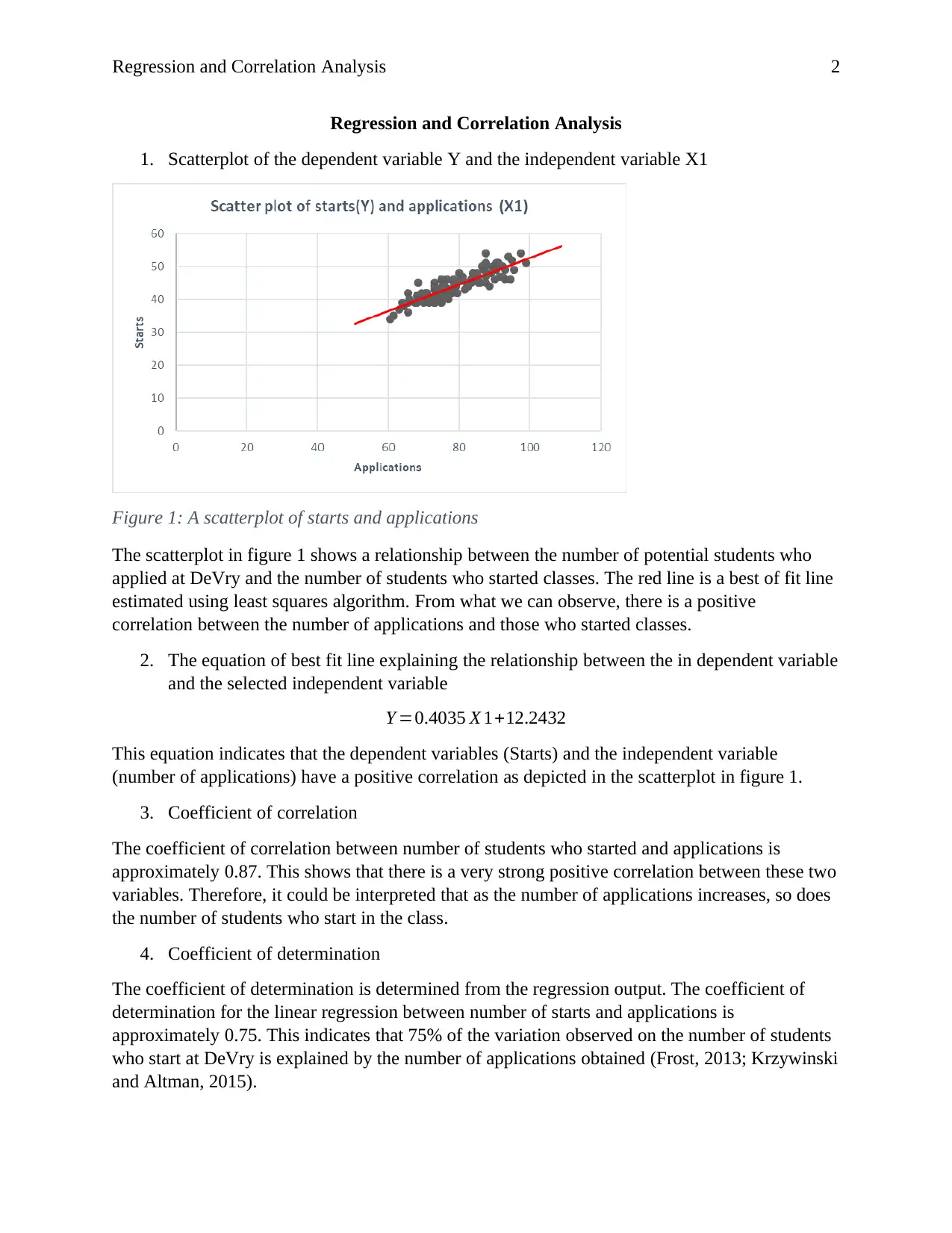
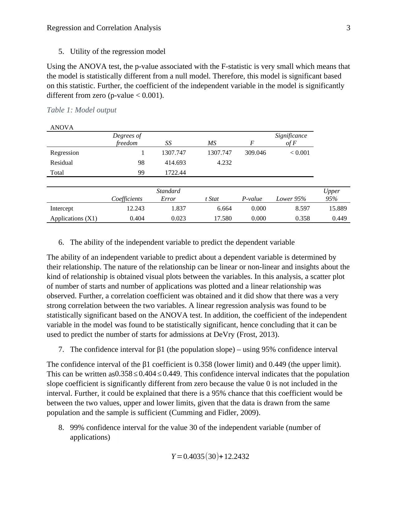
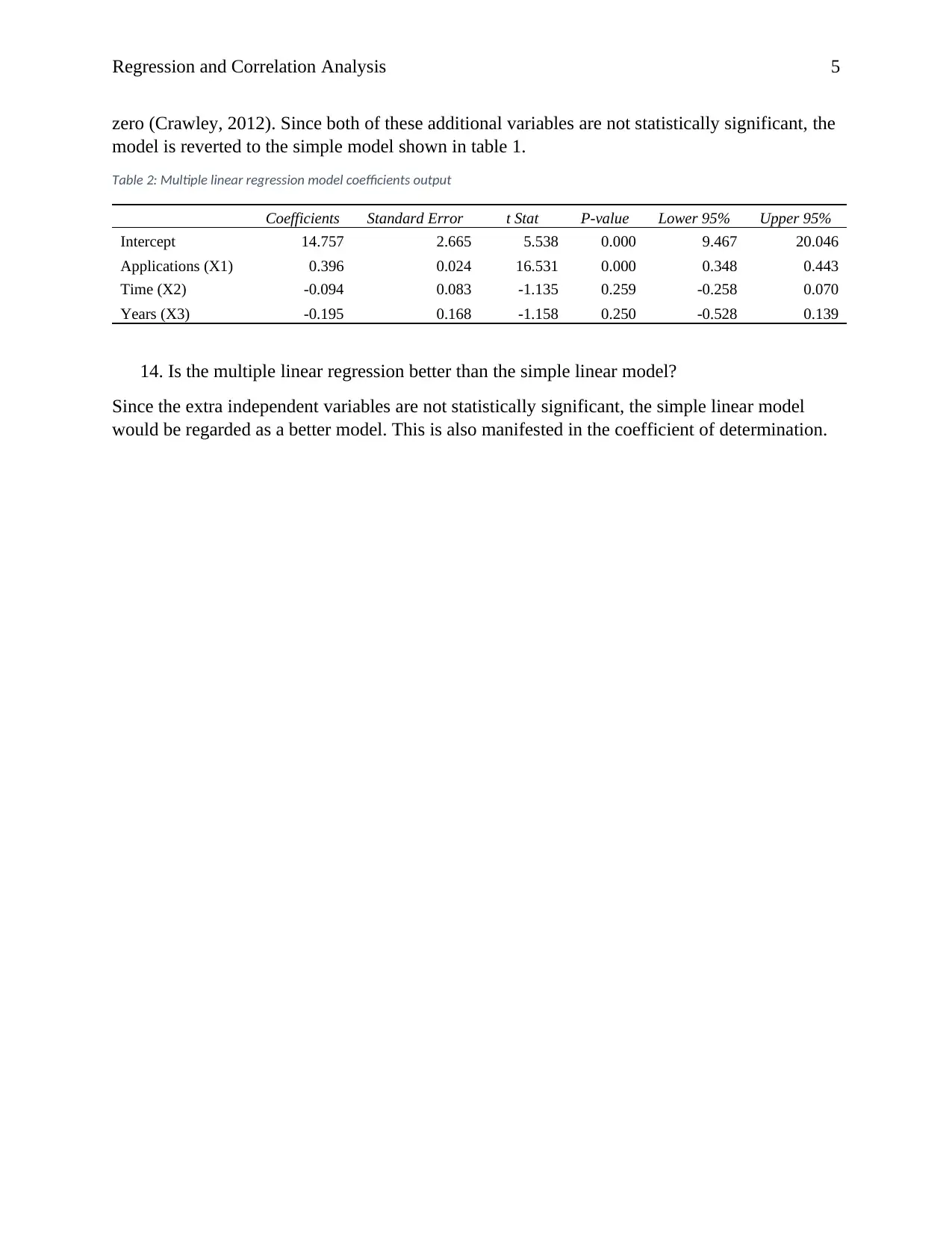
This report presents a regression and correlation analysis of DeVry admissions data, focusing on the relationship between the number of student applications and the number of students who started classes. The analysis includes a scatterplot visualization and the determination of the best-fit line equation. The coefficient of correlation and the coefficient of determination are calculated and interpreted to assess the strength and explanatory power of the relationship. The report also examines the utility of the regression model using ANOVA and t-tests, determining the statistical significance of the model and its independent variables. Confidence intervals for the slope coefficient and predicted values are calculated, providing insights into the reliability of the model's predictions. Furthermore, a multiple linear regression model is explored, comparing its performance to the simple linear model and assessing the significance of additional independent variables such as time spent with potential students and years of experience of the admissions advisors.

Regression and Correlation Analysis 1
Regression and Correlation Analysis
Name
Course Number
Date
Faculty Name

Regression and Correlation Analysis 2
Regression and Correlation Analysis
1. Scatterplot of the dependent variable Y and the independent variable X1
Figure 1: A scatterplot of starts and applications
The scatterplot in figure 1 shows a relationship between the number of potential students who
applied at DeVry and the number of students who started classes. The red line is a best of fit line
estimated using least squares algorithm. From what we can observe, there is a positive
correlation between the number of applications and those who started classes.
2. The equation of best fit line explaining the relationship between the in dependent variable
and the selected independent variable
Y =0.4035 X 1+12.2432
This equation indicates that the dependent variables (Starts) and the independent variable
(number of applications) have a positive correlation as depicted in the scatterplot in figure 1.
3. Coefficient of correlation
The coefficient of correlation between number of students who started and applications is
approximately 0.87. This shows that there is a very strong positive correlation between these two
variables. Therefore, it could be interpreted that as the number of applications increases, so does
the number of students who start in the class.
4. Coefficient of determination
The coefficient of determination is determined from the regression output. The coefficient of
determination for the linear regression between number of starts and applications is
approximately 0.75. This indicates that 75% of the variation observed on the number of students
who start at DeVry is explained by the number of applications obtained (Frost, 2013; Krzywinski
and Altman, 2015).

Regression and Correlation Analysis 3
5. Utility of the regression model
Using the ANOVA test, the p-value associated with the F-statistic is very small which means that
the model is statistically different from a null model. Therefore, this model is significant based
on this statistic. Further, the coefficient of the independent variable in the model is significantly
different from zero (p-value < 0.001).
Table 1: Model output
ANOVA
Degrees of
freedom SS MS F
Significance
of F
Regression 1 1307.747 1307.747 309.046 < 0.001
Residual 98 414.693 4.232
Total 99 1722.44
Coefficients
Standard
Error t Stat P-value Lower 95%
Upper
95%
Intercept 12.243 1.837 6.664 0.000 8.597 15.889
Applications (X1) 0.404 0.023 17.580 0.000 0.358 0.449
6. The ability of the independent variable to predict the dependent variable
The ability of an independent variable to predict about a dependent variable is determined by
their relationship. The nature of the relationship can be linear or non-linear and insights about the
kind of relationship is obtained visual plots between the variables. In this analysis, a scatter plot
of number of starts and number of applications was plotted and a linear relationship was
observed. Further, a correlation coefficient was obtained and it did show that there was a very
strong correlation between the two variables. A linear regression analysis was found to be
statistically significant based on the ANOVA test. In addition, the coefficient of the independent
variable in the model was found to be statistically significant, hence concluding that it can be
used to predict the number of starts for admissions at DeVry (Frost, 2013).
7. The confidence interval for β1 (the population slope) – using 95% confidence interval
The confidence interval of the β1 coefficient is 0.358 (lower limit) and 0.449 (the upper limit).
This can be written as0.358 ≤ 0.404 ≤ 0.449. This confidence interval indicates that the population
slope coefficient is significantly different from zero because the value 0 is not included in the
interval. Further, it could be explained that there is a 95% chance that this coefficient would be
between the two values, upper and lower limits, given that the data is drawn from the same
population and the sample is sufficient (Cumming and Fidler, 2009).
8. 99% confidence interval for the value 30 of the independent variable (number of
applications)
Y =0.4035(30)+12.2432

Regression and Correlation Analysis 4
Number of starts (Y) for 30 applications would be 24.3482 which is approximately 25
students.
The confidence interval for the predicted value are calculated using the confidence
intervals of the model coefficients.
Lower interval: 0. 35 8 ( 30 ) +8.597=19.337
Upper interval: 0. 449 ( 30 ) +15.889=29.359
This interval indicates that if the same study is conducted again using the same
population, the predicted number of students starting given that there were 30
applications would be between the lower and upper intervals at 99% confidence level.
9. 99% prediction interval
The 99% predict intervals for this estimates would be calculated as shown below:
¿ 24.3482 ±2.057∗2.575
¿ 24.3482 ±5.2968
¿ [19.0514 , 29.645]
These values mean that there is 99% confidence that the number of start at DeVry assuming that
30 students sent their applications would be between approximately 20 and 30.
10. Values of the dependent variable for values of the independent variable that are outside
the range of sample value
Given the confidence interval, the values which are beyond this limits could be said to be from a
different population apart from the one which was sampled. In other words, these can be
determined as outliers in the population.
11. Multiple linear regression
Y =14.757 +0.396 X 1−0.094 X 2−0.195 X 2
12. Utility test using F-statistic
The model is statistically significant compared to the null model (p-value < 0.001).
13. T-test on the independent variables
Application is the only statistically significant independent variable with a p-value associated
with the t-test that is less than 5% significance level. The model coefficients of Time (p-value =
0.2592) and Years (p-value = 0.2497) independent variables are not significantly different from

Regression and Correlation Analysis 5
zero (Crawley, 2012). Since both of these additional variables are not statistically significant, the
model is reverted to the simple model shown in table 1.
Table 2: Multiple linear regression model coefficients output
Coefficients Standard Error t Stat P-value Lower 95% Upper 95%
Intercept 14.757 2.665 5.538 0.000 9.467 20.046
Applications (X1) 0.396 0.024 16.531 0.000 0.348 0.443
Time (X2) -0.094 0.083 -1.135 0.259 -0.258 0.070
Years (X3) -0.195 0.168 -1.158 0.250 -0.528 0.139
14. Is the multiple linear regression better than the simple linear model?
Since the extra independent variables are not statistically significant, the simple linear model
would be regarded as a better model. This is also manifested in the coefficient of determination.

Regression and Correlation Analysis 6
References
Crawley, M. J. (2012) ‘Regression’, in The R Book, pp. 449–497. doi:
10.1002/9781118448908.ch10.
Cumming, G. and Fidler, F. (2009) ‘Confidence Intervals’, Zeitschrift für Psychologie / Journal
of Psychology, 217(1), pp. 15–26. doi: 10.1027/0044-3409.217.1.15.
Frost, J. (2013) Regression Analysis: How Do I Interpret R-squared and Assess the Goodness-
of-Fit?, Regression Analysis. Available at: http://blog.minitab.com/blog/adventures-in-statistics-
2/regression-analysis-how-do-i-interpret-r-squared-and-assess-the-goodness-of-fit.
Krzywinski, M. and Altman, N. (2015) ‘Points of Significance: Multiple linear regression’,
Nature Methods, pp. 1103–1104. doi: 10.1038/nmeth.3665.