Statistical Analysis of Consumer Behavior: Regression Homework

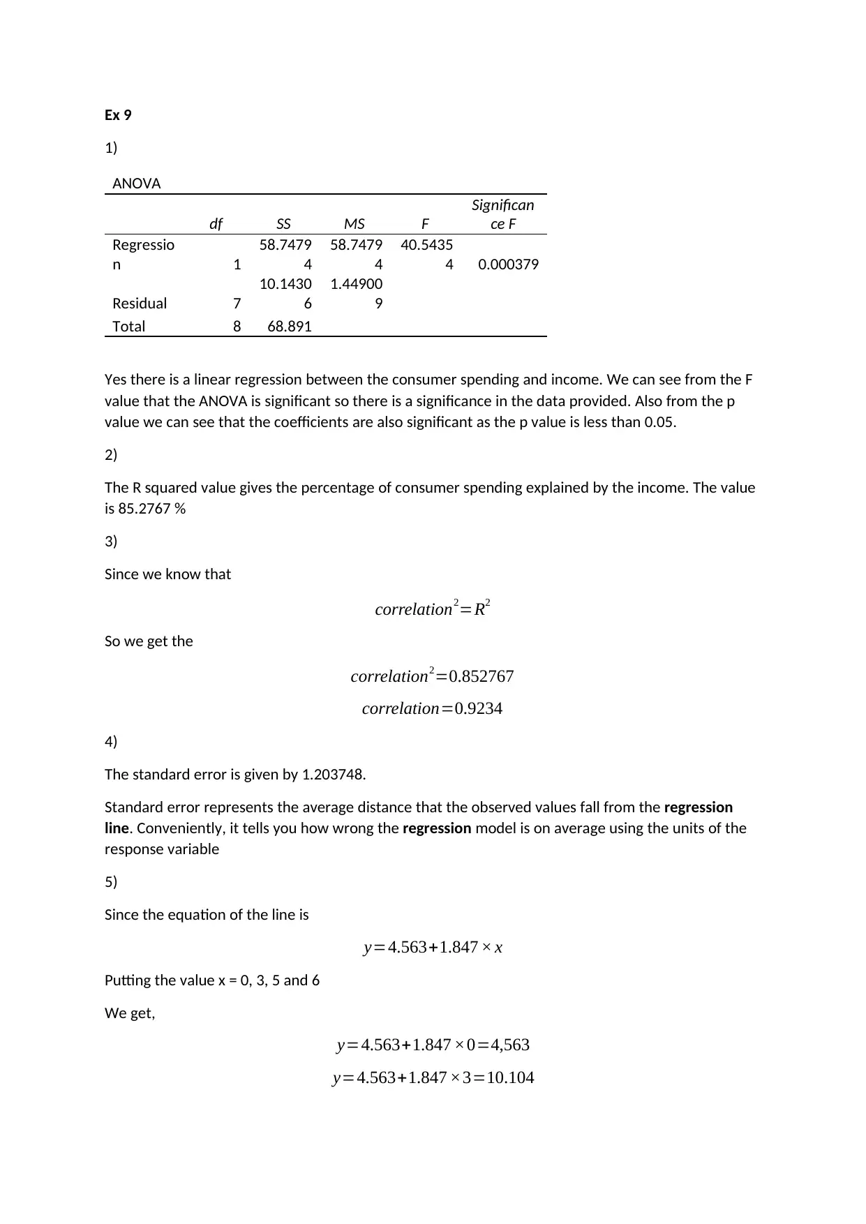
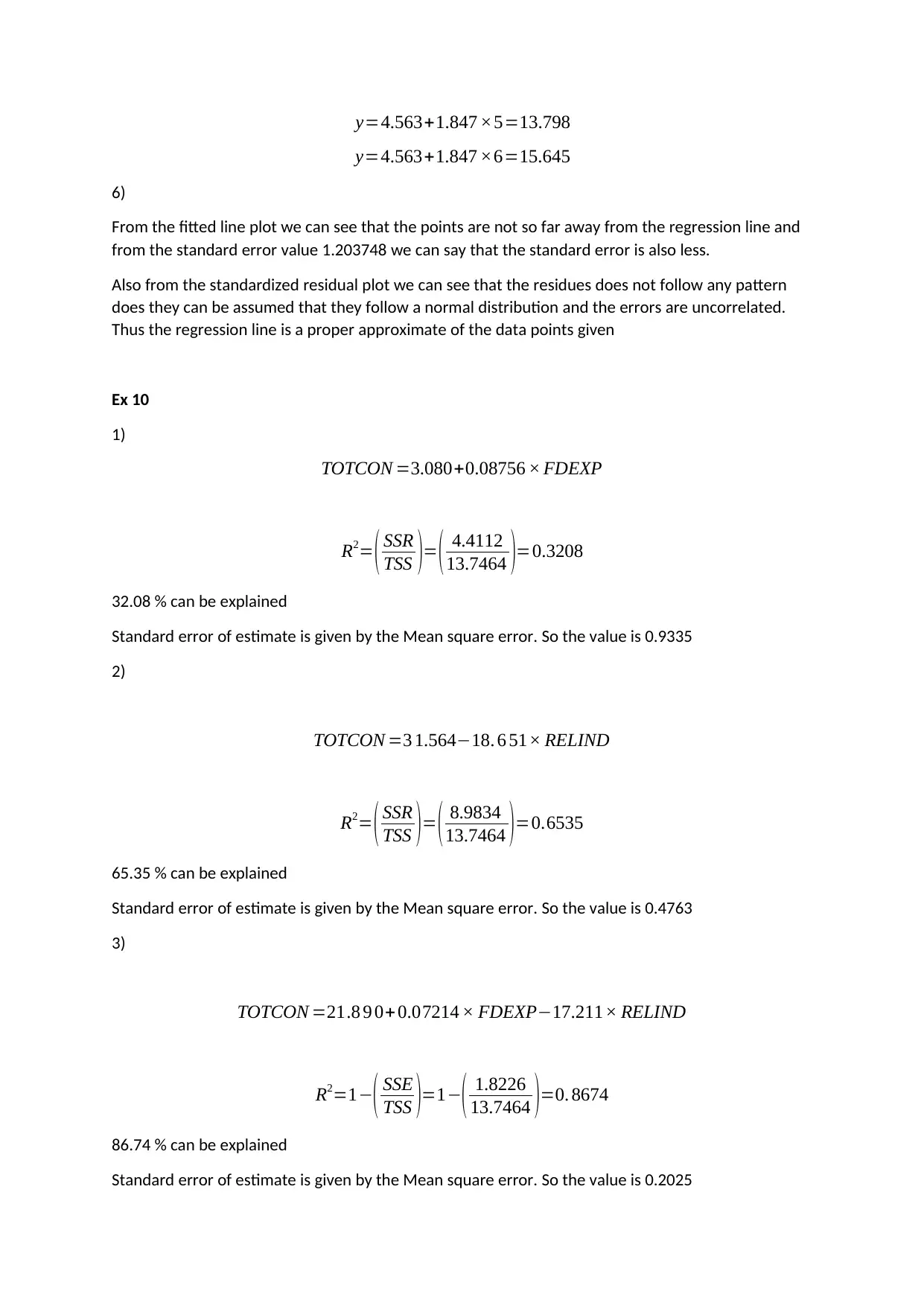
This document presents solutions to a statistics homework assignment. The first part of the solution analyzes the linear regression between consumer spending and income, including ANOVA results, R-squared value interpretation, correlation calculation, standard error analysis, and predicted values based on the regression equation. The second part explores multiple regression models to explain total meat consumption, evaluating the explanatory power of different independent variables like food expenditure and the ratio of consumer price indexes. The document provides detailed calculations and interpretations of statistical measures such as R-squared and standard error, offering a comprehensive understanding of the relationships between variables and the effectiveness of different regression models.

Ex 9
1)
ANOVA
df SS MS F
Significan
ce F
Regressio
n 1
58.7479
4
58.7479
4
40.5435
4 0.000379
Residual 7
10.1430
6
1.44900
9
Total 8 68.891
Yes there is a linear regression between the consumer spending and income. We can see from the F
value that the ANOVA is significant so there is a significance in the data provided. Also from the p
value we can see that the coefficients are also significant as the p value is less than 0.05.
2)
The R squared value gives the percentage of consumer spending explained by the income. The value
is 85.2767 %
3)
Since we know that
correlation2=R2
So we get the
correlation2=0.852767
correlation=0.9234
4)
The standard error is given by 1.203748.
Standard error represents the average distance that the observed values fall from the regression
line. Conveniently, it tells you how wrong the regression model is on average using the units of the
response variable
5)
Since the equation of the line is
y=4.563+1.847 × x
Putting the value x = 0, 3, 5 and 6
We get,
y=4.563+1.847 ×0=4,563
y=4.563+1.847 ×3=10.104

y=4.563+1.847 ×5=13.798
y=4.563+1.847 ×6=15.645
6)
From the fitted line plot we can see that the points are not so far away from the regression line and
from the standard error value 1.203748 we can say that the standard error is also less.
Also from the standardized residual plot we can see that the residues does not follow any pattern
does they can be assumed that they follow a normal distribution and the errors are uncorrelated.
Thus the regression line is a proper approximate of the data points given
Ex 10
1)
TOTCON =3.080+0.08756 × FDEXP
R2= ( SSR
TSS )= ( 4.4112
13.7464 )=0.3208
32.08 % can be explained
Standard error of estimate is given by the Mean square error. So the value is 0.9335
2)
TOTCON =3 1.564−18. 6 51× RELIND
R2= ( SSR
TSS )= ( 8.9834
13.7464 )=0.6535
65.35 % can be explained
Standard error of estimate is given by the Mean square error. So the value is 0.4763
3)
TOTCON =21.8 9 0+ 0.07214 × FDEXP−17.211× RELIND
R2=1−( SSE
TSS )=1−( 1.8226
13.7464 )=0. 8674
86.74 % can be explained
Standard error of estimate is given by the Mean square error. So the value is 0.2025

4)
Total consumption of Meat will be better explained by both Consumption expenditure on food and
ratio of consumer price indexes of processed meat to all meats. Since when both of the independent
variables are used we are getting a better coefficient of determination.