Regression Analysis Homework: Model Significance and Variable Impacts

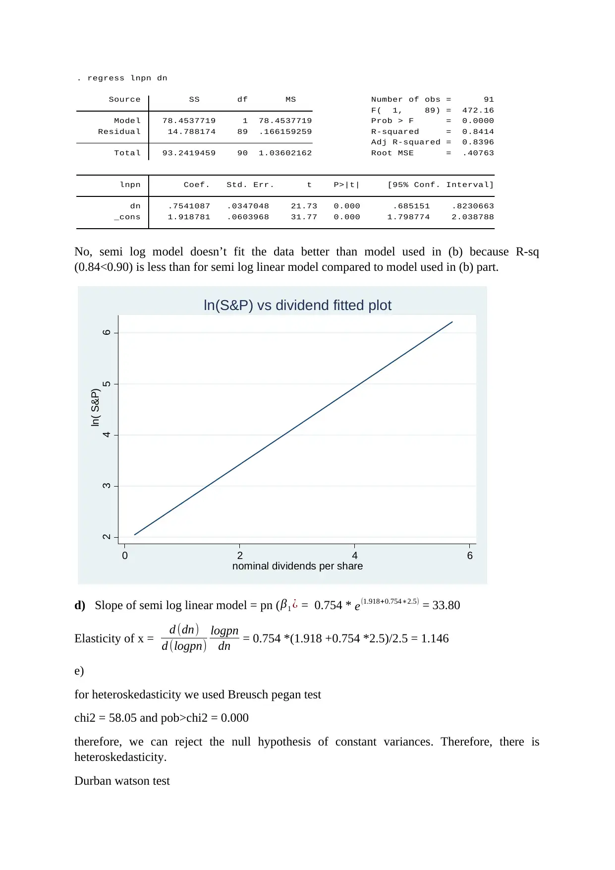
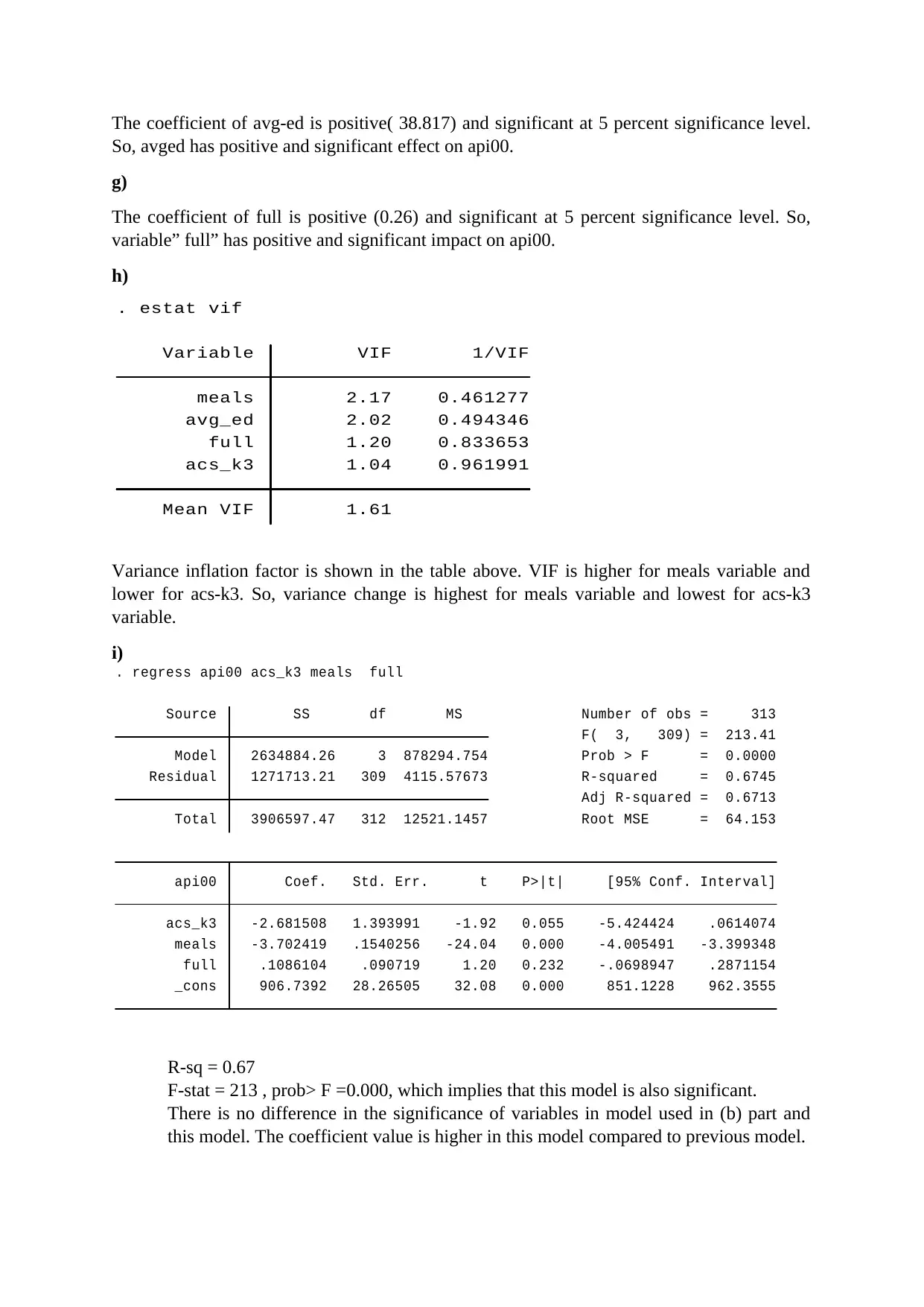
This document presents a solution to a regression analysis homework assignment, covering various aspects of statistical modeling and econometrics. The assignment involves analyzing the relationship between S&P and dividend per share, evaluating the fit of different models (linear and semi-log), ...Read More

Assignment
Que:1
Fitted plot between S&P and dividend per share is as:
a)
b)
_cons -1.467476 1.496313 -0.98 0.329 -4.440618 1.505665
dn 25.44639 .8598009 29.60 0.000 23.73799 27.1548
pn Coef. Std. Err. t P>|t| [95% Conf. Interval]
Total 98407.002 90 1093.41113 Root MSE = 10.099
Adj R-squared = 0.9067
Residual 9076.77895 89 101.98628 R-squared = 0.9078
Model 89330.223 1 89330.223 Prob > F = 0.0000
F( 1, 89) = 875.90
Source SS df MS Number of obs = 91
regress pn dn
The slope coefficient is 25.44 and intercept is -1.46. p- value for slope coefficient is 0.000
which is significant at even 1 percent significance level. Therefore, we can say that there is
positive and linear relationship between S& P and dividend.
c) semi log linear model
log ( pn )=β0 + β1 dn+u
Estimates of semi log linear model are:

_cons 1.918781 .0603968 31.77 0.000 1.798774 2.038788
dn .7541087 .0347048 21.73 0.000 .685151 .8230663
lnpn Coef. Std. Err. t P>|t| [95% Conf. Interval]
Total 93.2419459 90 1.03602162 Root MSE = .40763
Adj R-squared = 0.8396
Residual 14.788174 89 .166159259 R-squared = 0.8414
Model 78.4537719 1 78.4537719 Prob > F = 0.0000
F( 1, 89) = 472.16
Source SS df MS Number of obs = 91
. regress lnpn dn
No, semi log model doesn’t fit the data better than model used in (b) because R-sq
(0.84<0.90) is less than for semi log linear model compared to model used in (b) part.
2 3 4 5 6
ln( S&P)
0 2 4 6
nominal dividends per share
ln(S&P) vs dividend fitted plot
d) Slope of semi log linear model = pn (β1 ¿ = 0.754 * e(1.918+0.754∗2.5) = 33.80
Elasticity of x = d (dn)
d (logpn)
logpn
dn = 0.754 *(1.918 +0.754 *2.5)/2.5 = 1.146
e)
for heteroskedasticity we used Breusch pegan test
chi2 = 58.05 and pob>chi2 = 0.000
therefore, we can reject the null hypothesis of constant variances. Therefore, there is
heteroskedasticity.
Durban watson test

Chi2 = 493.67 and p-value = 0.000
So, we can reject the null hypothesis of no serial autocorrelation and conclude that thereal is a
serial autocorrelation problem in the model.
Que:4
a)
_cons 753.4775 42.37355 17.78 0.000 670.0824 836.8726
full .2460843 .0921666 2.67 0.008 .0646918 .4274768
avg_ed 38.81789 8.167805 4.75 0.000 22.74288 54.89289
meals -3.016457 .2181518 -13.83 0.000 -3.445801 -2.587114
acs_k3 -2.557612 1.363709 -1.88 0.062 -5.241519 .1262939
api00 Coef. Std. Err. t P>|t| [95% Conf. Interval]
Total 3741706.3 297 12598.3377 Root MSE = 61.705
Adj R-squared = 0.6978
Residual 1115599.13 293 3807.50558 R-squared = 0.7018
Model 2626107.16 4 656526.79 Prob > F = 0.0000
F( 4, 293) = 172.43
Source SS df MS Number of obs = 298
. regress api00 acs_k3 meals avg_ed full
b)
R-sq = 0.70. this means that 70 percent variation in variable api00 can be explained by this
model.
c)
F-stat = 172.493, , p-value = 0.000
p- value is less than 0.05. this means that our model is significant or valid.
d)
the coefficient of acs_k3 is negative(-2.557), but not significant at 5 percent significance
level. If p-value is less than 0.05, then only a coefficient is significant at 5 percent
significance level.
e)
The coefficient of meals is negative (-3.017) and significant at 5 percent significance level as
p-value is less than 0.05. So, meals has negative and significant impact on api00.
f)

The coefficient of avg-ed is positive( 38.817) and significant at 5 percent significance level.
So, avged has positive and significant effect on api00.
g)
The coefficient of full is positive (0.26) and significant at 5 percent significance level. So,
variable” full” has positive and significant impact on api00.
h)
Mean VIF 1.61
acs_k3 1.04 0.961991
full 1.20 0.833653
avg_ed 2.02 0.494346
meals 2.17 0.461277
Variable VIF 1/VIF
. estat vif
Variance inflation factor is shown in the table above. VIF is higher for meals variable and
lower for acs-k3. So, variance change is highest for meals variable and lowest for acs-k3
variable.
i)
_cons 906.7392 28.26505 32.08 0.000 851.1228 962.3555
full .1086104 .090719 1.20 0.232 -.0698947 .2871154
meals -3.702419 .1540256 -24.04 0.000 -4.005491 -3.399348
acs_k3 -2.681508 1.393991 -1.92 0.055 -5.424424 .0614074
api00 Coef. Std. Err. t P>|t| [95% Conf. Interval]
Total 3906597.47 312 12521.1457 Root MSE = 64.153
Adj R-squared = 0.6713
Residual 1271713.21 309 4115.57673 R-squared = 0.6745
Model 2634884.26 3 878294.754 Prob > F = 0.0000
F( 3, 309) = 213.41
Source SS df MS Number of obs = 313
. regress api00 acs_k3 meals full
R-sq = 0.67
F-stat = 213 , prob> F =0.000, which implies that this model is also significant.
There is no difference in the significance of variables in model used in (b) part and
this model. The coefficient value is higher in this model compared to previous model.

R-sq is less than for this model compared to model used in (b) part. So, omitting the
variable has significant impact on model. Therefore, model used in (b) part is better
model than this model.