Analyzing CEO Salaries and Commodity Prices: An Economic Project
VerifiedAdded on 2021/06/07
|15
|2850
|227
Project
AI Summary
This project undertakes a comprehensive economic analysis, beginning with a multiple ordinary least squares (OLS) regression model to predict CEO salaries, incorporating variables such as return on assets, firm size, volatility, CEO age, gender, and board independence. The model's performance is evaluated through R-squared, adjusted R-squared, ANOVA, and parameter estimates. The second part of the project delves into commodity price analysis, focusing on wheat, sugar, and chicken prices from 2019 to 2021. It examines weak-form efficiency and utilizes descriptive statistics, including histograms and time series plots, to understand price behavior. Furthermore, the project employs an autoregressive (AR) model to forecast future price movements, providing model statistics and interpretations for each commodity.
Part 1:
Model Description:
Multiple OLS is a statistical method that predicts the outcome of a response variable by
combining many explanatory variables. MLR targets to model the linear relationship between
explanatory variables accompanied by the response, variable.
To predict log salary for the CEO, we used a multiple regression model with the following
variables: return for assets for the firm; the log of total assets of the company; volatility
measured by the daily return; the age of the CEO for the firm, CEO female and extent of
independent directors.
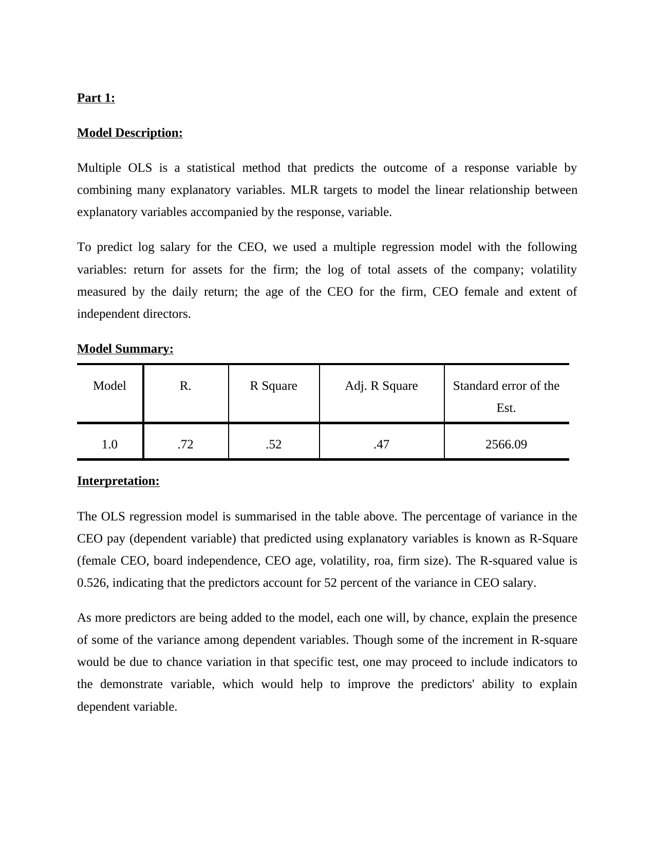
Model Summary:
Model R. R Square Adj. R Square Standard error of the
Est.
1.0 .72 .52 .47 2566.09
Interpretation:
The OLS regression model is summarised in the table above. The percentage of variance in the
CEO pay (dependent variable) that predicted using explanatory variables is known as R-Square
(female CEO, board independence, CEO age, volatility, roa, firm size). The R-squared value is
0.526, indicating that the predictors account for 52 percent of the variance in CEO salary.
As more predictors are being added to the model, each one will, by chance, explain the presence
of some of the variance among dependent variables. Though some of the increment in R-square
would be due to chance variation in that specific test, one may proceed to include indicators to
the demonstrate variable, which would help to improve the predictors' ability to explain
dependent variable.
Model Description:
Multiple OLS is a statistical method that predicts the outcome of a response variable by
combining many explanatory variables. MLR targets to model the linear relationship between
explanatory variables accompanied by the response, variable.
To predict log salary for the CEO, we used a multiple regression model with the following
variables: return for assets for the firm; the log of total assets of the company; volatility
measured by the daily return; the age of the CEO for the firm, CEO female and extent of
independent directors.
Model Summary:
Model R. R Square Adj. R Square Standard error of the
Est.
1.0 .72 .52 .47 2566.09
Interpretation:
The OLS regression model is summarised in the table above. The percentage of variance in the
CEO pay (dependent variable) that predicted using explanatory variables is known as R-Square
(female CEO, board independence, CEO age, volatility, roa, firm size). The R-squared value is
0.526, indicating that the predictors account for 52 percent of the variance in CEO salary.
As more predictors are being added to the model, each one will, by chance, explain the presence
of some of the variance among dependent variables. Though some of the increment in R-square
would be due to chance variation in that specific test, one may proceed to include indicators to
the demonstrate variable, which would help to improve the predictors' ability to explain
dependent variable.
Paraphrase This Document
Need a fresh take? Get an instant paraphrase of this document with our AI Paraphraser
Adjusted R-square is attempt to quantify R-squared for the population with a more accurate
value. In our model, the modified R square value is 0.47. The standard deviation’s value of the
error term is 2566.09, and the standard error of the estimation is 2566.09.
ANOVA:
Models Sum of Squares Df Mean Square F Sig.
Regression. 415884877.32 6.00 69314146.22 10.52 .00
Residual. 375335876.67 57.00 6584839.94
Total. 791220754.00 63.00
Interpretation:
The result of the ANOVA is shown in the table above. In the second column, we are having a
source of variation, The total SS is 791220754.00, which is divided into regression and residual
parts, the SS for residual is 375335876.67 with 57 degrees of freedom while SS for regression is
415884877.32 having 6 degrees of freedom. MS are calculated so that you can test the
importance of the predictors for the model by dividing by the Mean Square Regression with
Mean Square Residual and computing F ratio.
The p-value which is linked with the F value is 0, which is very small. Thus we can assume that
the independent variables is accurately predicting the dependent variable since the p-value is less
than alpha 0.05. We would argue that the factors female CEO, board independence, CEO age,
volatility, roa, and firm size can be used to predict CEO pay with reasonable accuracy.
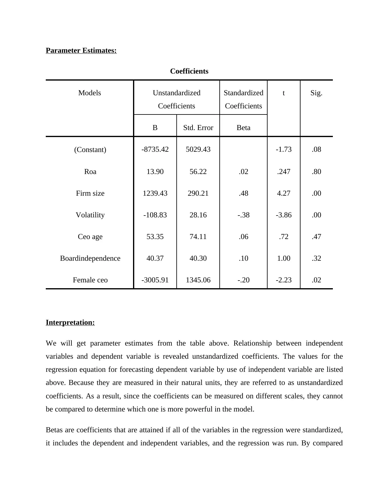
Parameter Estimates:
Coefficients
Models Unstandardized
Coefficients
Standardized
Coefficients
t Sig.
B Std. Error Beta
(Constant) -8735.42 5029.43 -1.73 .08
Roa 13.90 56.22 .02 .247 .80
Firm size 1239.43 290.21 .48 4.27 .00
Volatility -108.83 28.16 -.38 -3.86 .00
Ceo age 53.35 74.11 .06 .72 .47
Boardindependence 40.37 40.30 .10 1.00 .32
Female ceo -3005.91 1345.06 -.20 -2.23 .02
Interpretation:
We will get parameter estimates from the table above. Relationship between independent
variables and dependent variable is revealed unstandardized coefficients. The values for the
regression equation for forecasting dependent variable by use of independent variable are listed
above. Because they are measured in their natural units, they are referred to as unstandardized
coefficients. As a result, since the coefficients can be measured on different scales, they cannot
be compared to determine which one is more powerful in the model.
Betas are coefficients that are attained if all of the variables in the regression were standardized,
it includes the dependent and independent variables, and the regression was run. By compared
Coefficients
Models Unstandardized
Coefficients
Standardized
Coefficients
t Sig.
B Std. Error Beta
(Constant) -8735.42 5029.43 -1.73 .08
Roa 13.90 56.22 .02 .247 .80
Firm size 1239.43 290.21 .48 4.27 .00
Volatility -108.83 28.16 -.38 -3.86 .00
Ceo age 53.35 74.11 .06 .72 .47
Boardindependence 40.37 40.30 .10 1.00 .32
Female ceo -3005.91 1345.06 -.20 -2.23 .02
Interpretation:
We will get parameter estimates from the table above. Relationship between independent
variables and dependent variable is revealed unstandardized coefficients. The values for the
regression equation for forecasting dependent variable by use of independent variable are listed
above. Because they are measured in their natural units, they are referred to as unstandardized
coefficients. As a result, since the coefficients can be measured on different scales, they cannot
be compared to determine which one is more powerful in the model.
Betas are coefficients that are attained if all of the variables in the regression were standardized,
it includes the dependent and independent variables, and the regression was run. By compared
⊘ This is a preview!⊘
Do you want full access?
Subscribe today to unlock all pages.
Trusted by 1+ million students worldwide
size of coefficients to check which one has more of an effect by institutionalizing factors
sometime recently running regression.
These estimates show how much of an increase in CEO pay can be expected by a one-unit
increase in the predictor, for example, a one-unit increase in the firm size would result in a
1239.43 increase in CEO pay, similarly, a one-unit increase in the firm's return on assets percent
would result in a 13.90 increase in CEO pay. Statistically important coefficients have p-values
less than alpha. Firm size, volatility, and female CEO are all important coefficients in our model.
Because the p-value is greater than .05, therefore, coefficients for roa, CEO age, and board
independence are not statistically significant at the 0.05 level.
Part 2:
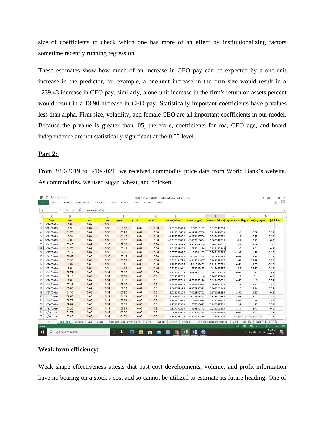
From 3/10/2019 to 3/10/2021, we received commodity price data from World Bank’s website.
As commodities, we used sugar, wheat, and chicken.
Weak form efficiency:
Weak shape effectiveness attests that past cost developments, volume, and profit information
have no bearing on a stock's cost and so cannot be utilized to estimate its future heading. One of
sometime recently running regression.
These estimates show how much of an increase in CEO pay can be expected by a one-unit
increase in the predictor, for example, a one-unit increase in the firm size would result in a
1239.43 increase in CEO pay, similarly, a one-unit increase in the firm's return on assets percent
would result in a 13.90 increase in CEO pay. Statistically important coefficients have p-values
less than alpha. Firm size, volatility, and female CEO are all important coefficients in our model.
Because the p-value is greater than .05, therefore, coefficients for roa, CEO age, and board
independence are not statistically significant at the 0.05 level.
Part 2:
From 3/10/2019 to 3/10/2021, we received commodity price data from World Bank’s website.
As commodities, we used sugar, wheat, and chicken.
Weak form efficiency:
Weak shape effectiveness attests that past cost developments, volume, and profit information
have no bearing on a stock's cost and so cannot be utilized to estimate its future heading. One of
Paraphrase This Document
Need a fresh take? Get an instant paraphrase of this document with our AI Paraphraser
the three degrees of compelling advertise hypothesis is weak frame effectiveness (EMH). The
arbitrary walk hypothesis, moreover known as frail frame productivity, states that future security
costs are arbitrary and unaffected by past occasions. Advocates of weak frame effectiveness
accept that stock prices represent all current data, which past data has no bearing on current
showcase prices. Technical examination isn't considered exact by powerless frame adequacy, and
indeed basic analysis can be imperfect at times. Beating the showcase, especially within the brief
term, is subsequently amazingly troublesome due to low frame efficiency.
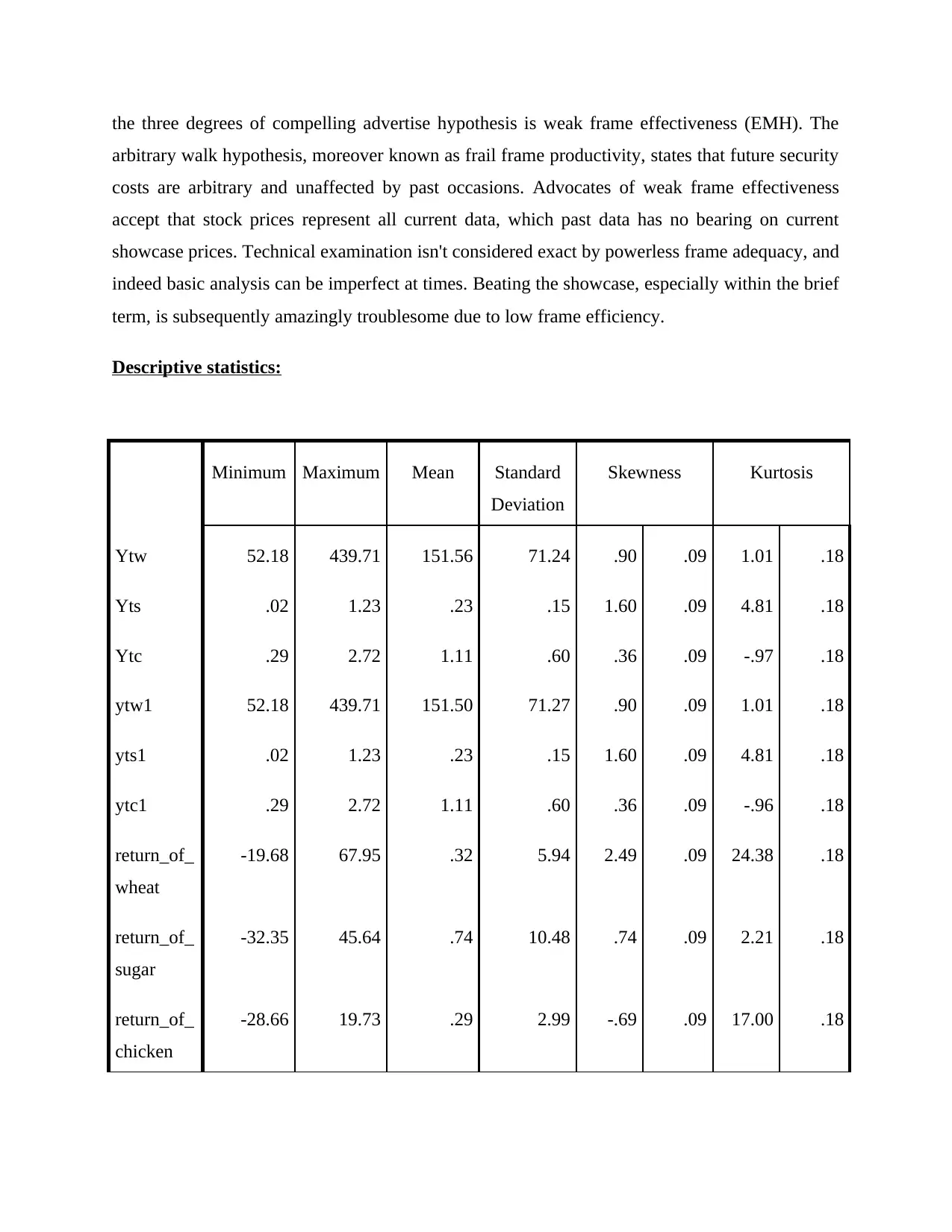
Descriptive statistics:
Minimum Maximum Mean Standard
Deviation
Skewness Kurtosis
Ytw 52.18 439.71 151.56 71.24 .90 .09 1.01 .18
Yts .02 1.23 .23 .15 1.60 .09 4.81 .18
Ytc .29 2.72 1.11 .60 .36 .09 -.97 .18
ytw1 52.18 439.71 151.50 71.27 .90 .09 1.01 .18
yts1 .02 1.23 .23 .15 1.60 .09 4.81 .18
ytc1 .29 2.72 1.11 .60 .36 .09 -.96 .18
return_of_
wheat
-19.68 67.95 .32 5.94 2.49 .09 24.38 .18
return_of_
sugar
-32.35 45.64 .74 10.48 .74 .09 2.21 .18
return_of_
chicken
-28.66 19.73 .29 2.99 -.69 .09 17.00 .18
arbitrary walk hypothesis, moreover known as frail frame productivity, states that future security
costs are arbitrary and unaffected by past occasions. Advocates of weak frame effectiveness
accept that stock prices represent all current data, which past data has no bearing on current
showcase prices. Technical examination isn't considered exact by powerless frame adequacy, and
indeed basic analysis can be imperfect at times. Beating the showcase, especially within the brief
term, is subsequently amazingly troublesome due to low frame efficiency.
Descriptive statistics:
Minimum Maximum Mean Standard
Deviation
Skewness Kurtosis
Ytw 52.18 439.71 151.56 71.24 .90 .09 1.01 .18
Yts .02 1.23 .23 .15 1.60 .09 4.81 .18
Ytc .29 2.72 1.11 .60 .36 .09 -.97 .18
ytw1 52.18 439.71 151.50 71.27 .90 .09 1.01 .18
yts1 .02 1.23 .23 .15 1.60 .09 4.81 .18
ytc1 .29 2.72 1.11 .60 .36 .09 -.96 .18
return_of_
wheat
-19.68 67.95 .32 5.94 2.49 .09 24.38 .18
return_of_
sugar
-32.35 45.64 .74 10.48 .74 .09 2.21 .18
return_of_
chicken
-28.66 19.73 .29 2.99 -.69 .09 17.00 .18
Interpretation:
The maximum and minimum price of wheat per kilogram from 2/1/2019 to 2/1/2021 are 439.71$
and 52.18$. Standard deviation computes the spread of a set of data. The greater value of
standard deviation, more data to be evenly distributed. Its value for wheat per kg is 71.24, the
degree and direction of asymmetry are measured by skewness. Asymmetric distribution, such as
a regular distribution, incorporates skewness of 0, while a skewed from the left distribution, such
as when the value of the mean is less than the median, contains a negative skewness, skewness
ranges from 0.90 to 0.09, while Kurtosis is a measure of tail extremity that reflects the existence
of outliers in any distribution or the proclivity of any distribution for production of outliers,
kurtosis ranges from 1.01 to 0.18. The maximum and minimum price of sugar per kilogram from
2/1/2019 to 2/1/2021 are 1.23$ and 0.02$. The standard deviation for sugar per kg is 0.15,
skewness ranges from 1.60 to 0.09, and similarly, kurtosis ranges from 4.81 to 0.18. The
maximum and minimum price of chicken per kilogram from 2/1/2019 to 2/1/2021 are 2.72$ and
0.29$. The standard deviation for chicken per kg is 0.60, skewness ranges from 0.36 to 0.09, and
similarly, kurtosis ranges from -0.97 to 0.18.
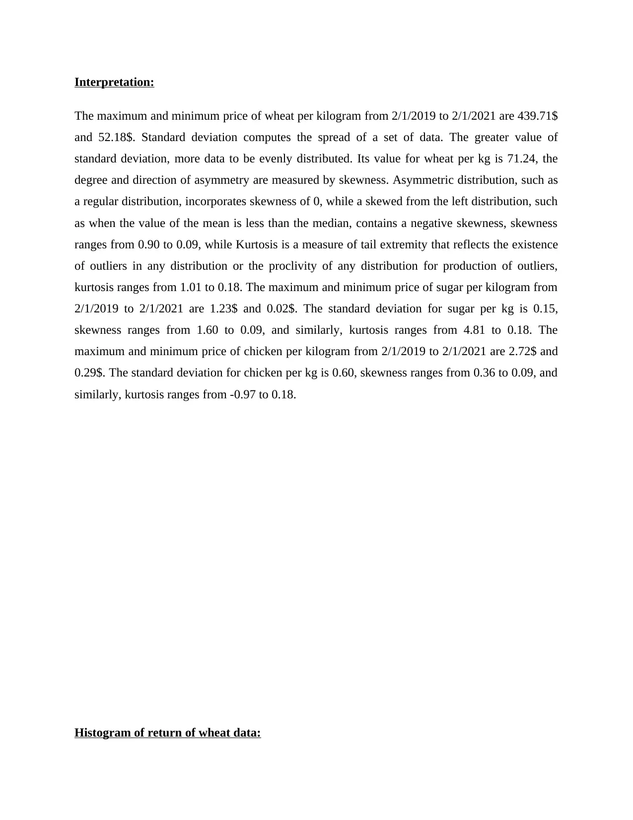
Histogram of return of wheat data:
The maximum and minimum price of wheat per kilogram from 2/1/2019 to 2/1/2021 are 439.71$
and 52.18$. Standard deviation computes the spread of a set of data. The greater value of
standard deviation, more data to be evenly distributed. Its value for wheat per kg is 71.24, the
degree and direction of asymmetry are measured by skewness. Asymmetric distribution, such as
a regular distribution, incorporates skewness of 0, while a skewed from the left distribution, such
as when the value of the mean is less than the median, contains a negative skewness, skewness
ranges from 0.90 to 0.09, while Kurtosis is a measure of tail extremity that reflects the existence
of outliers in any distribution or the proclivity of any distribution for production of outliers,
kurtosis ranges from 1.01 to 0.18. The maximum and minimum price of sugar per kilogram from
2/1/2019 to 2/1/2021 are 1.23$ and 0.02$. The standard deviation for sugar per kg is 0.15,
skewness ranges from 1.60 to 0.09, and similarly, kurtosis ranges from 4.81 to 0.18. The
maximum and minimum price of chicken per kilogram from 2/1/2019 to 2/1/2021 are 2.72$ and
0.29$. The standard deviation for chicken per kg is 0.60, skewness ranges from 0.36 to 0.09, and
similarly, kurtosis ranges from -0.97 to 0.18.
Histogram of return of wheat data:
⊘ This is a preview!⊘
Do you want full access?
Subscribe today to unlock all pages.
Trusted by 1+ million students worldwide
Interpretation:
The above figure tells us that histogram is following right-skewed distribution, a right-skewed
histogram has a left-of-center peak & a slow tapering to proper right side of graph. More the
mode is closer to left of graph and smaller than either the mean or the median, indicating that this
is a unimodal data set. The mean of rightly skewed data will be on the right side of the graph and
it will be higher than the median or mode. Diagram shows that there are large quantities of data
points that are larger than the mode, possibly outliers.
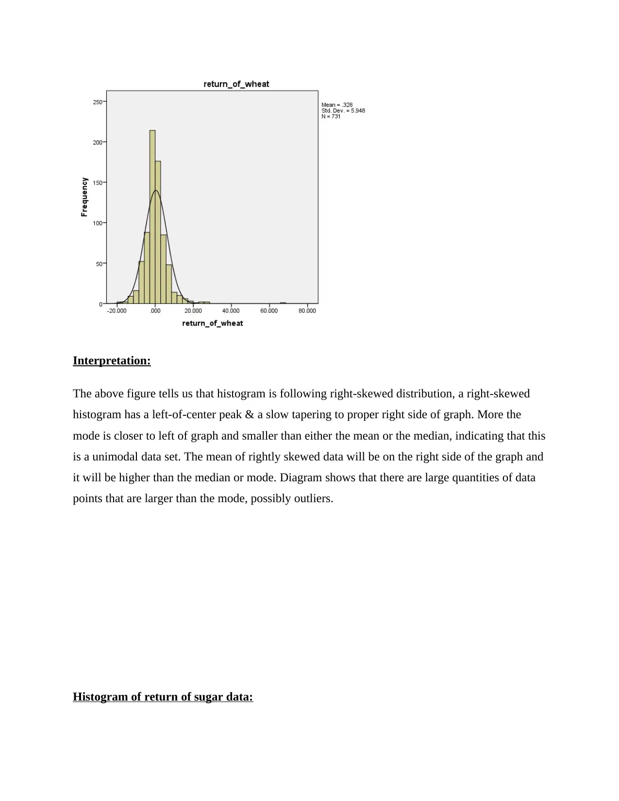
Histogram of return of sugar data:
The above figure tells us that histogram is following right-skewed distribution, a right-skewed
histogram has a left-of-center peak & a slow tapering to proper right side of graph. More the
mode is closer to left of graph and smaller than either the mean or the median, indicating that this
is a unimodal data set. The mean of rightly skewed data will be on the right side of the graph and
it will be higher than the median or mode. Diagram shows that there are large quantities of data
points that are larger than the mode, possibly outliers.
Histogram of return of sugar data:
Paraphrase This Document
Need a fresh take? Get an instant paraphrase of this document with our AI Paraphraser
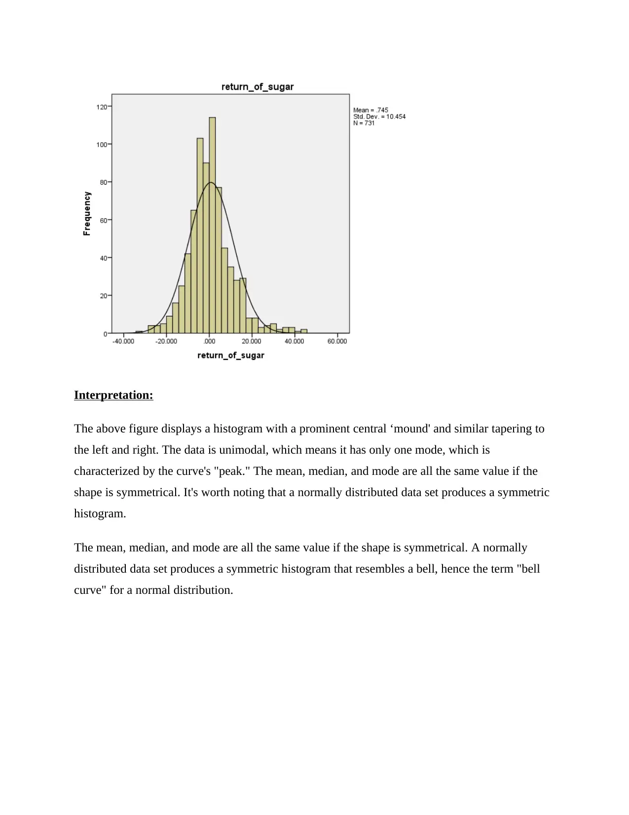
Interpretation:
The above figure displays a histogram with a prominent central ‘mound' and similar tapering to
the left and right. The data is unimodal, which means it has only one mode, which is
characterized by the curve's "peak." The mean, median, and mode are all the same value if the
shape is symmetrical. It's worth noting that a normally distributed data set produces a symmetric
histogram.
The mean, median, and mode are all the same value if the shape is symmetrical. A normally
distributed data set produces a symmetric histogram that resembles a bell, hence the term "bell
curve" for a normal distribution.
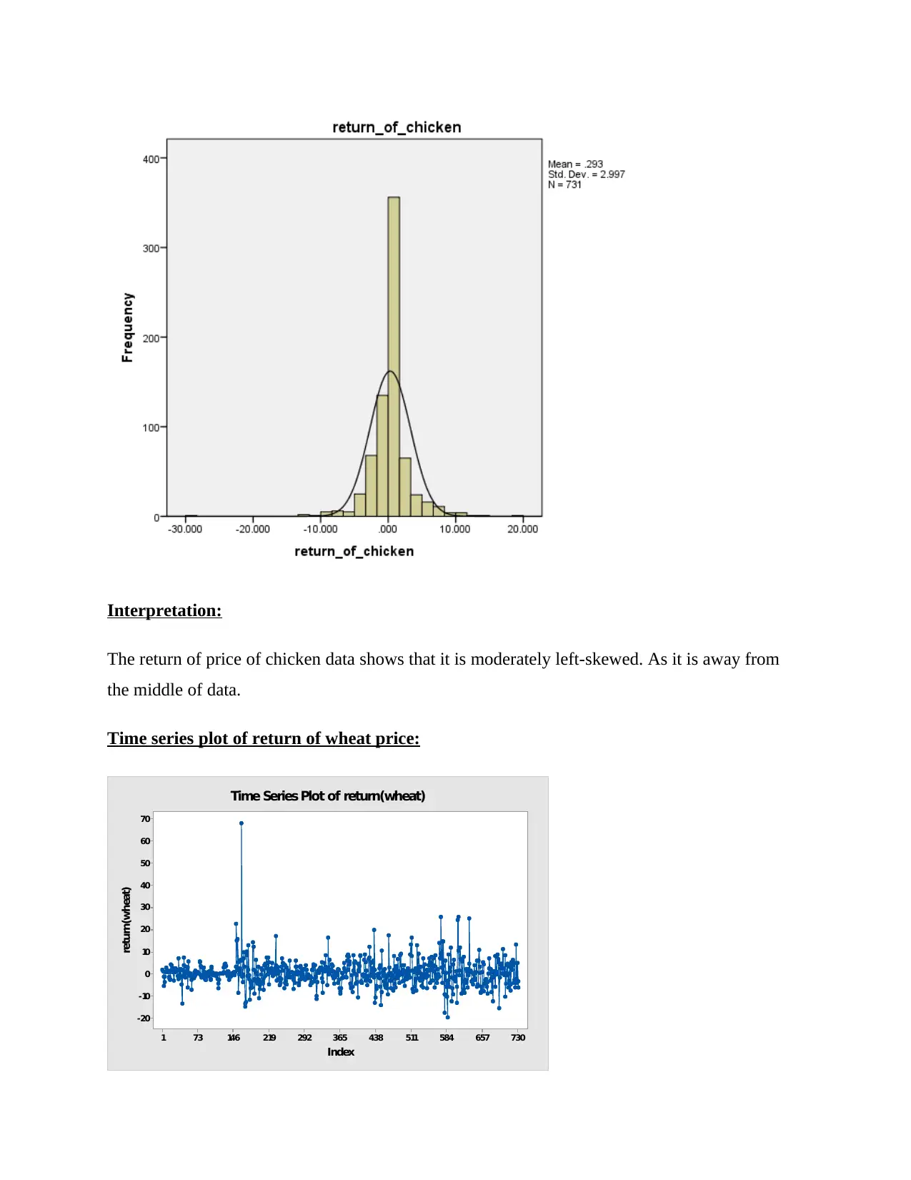
Interpretation:
The return of price of chicken data shows that it is moderately left-skewed. As it is away from
the middle of data.
Time series plot of return of wheat price:
730657584511438365292219146731
70
60
50
40
30
20
10
0
-10
-20
Index
return(wheat)
Time Series Plot of return(wheat)
The return of price of chicken data shows that it is moderately left-skewed. As it is away from
the middle of data.
Time series plot of return of wheat price:
730657584511438365292219146731
70
60
50
40
30
20
10
0
-10
-20
Index
return(wheat)
Time Series Plot of return(wheat)
⊘ This is a preview!⊘
Do you want full access?
Subscribe today to unlock all pages.
Trusted by 1+ million students worldwide
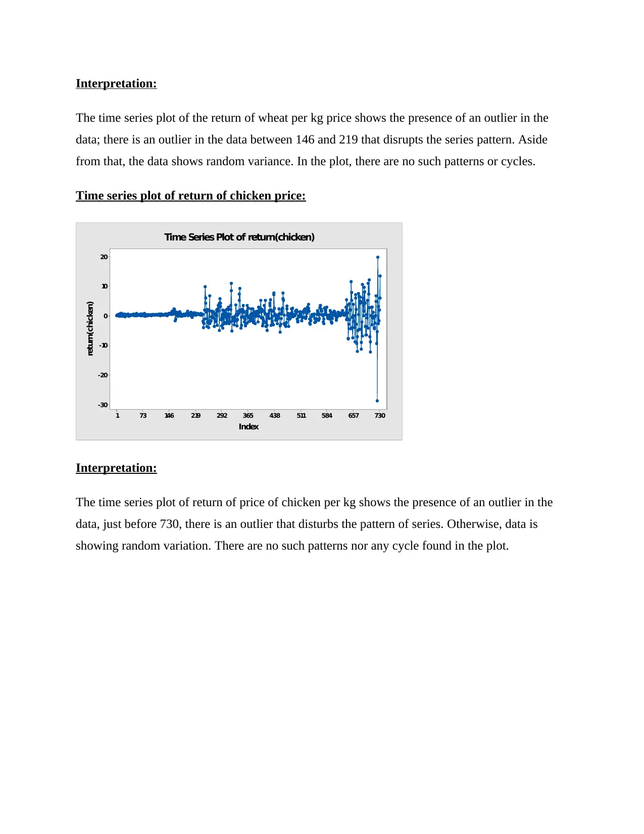
Interpretation:
The time series plot of the return of wheat per kg price shows the presence of an outlier in the
data; there is an outlier in the data between 146 and 219 that disrupts the series pattern. Aside
from that, the data shows random variance. In the plot, there are no such patterns or cycles.
Time series plot of return of chicken price:
730657584511438365292219146731
20
10
0
-10
-20
-30
Index
return(chicken)
Time Series Plot of return(chicken)
Interpretation:
The time series plot of return of price of chicken per kg shows the presence of an outlier in the
data, just before 730, there is an outlier that disturbs the pattern of series. Otherwise, data is
showing random variation. There are no such patterns nor any cycle found in the plot.
Paraphrase This Document
Need a fresh take? Get an instant paraphrase of this document with our AI Paraphraser
Time series plot of return of sugar price:
730657584511438365292219146731
50
40
30
20
10
0
-10
-20
-30
-40
Index
return(sugar)
Time Series Plot of return(sugar)
Interpretation:
You can see the Random variation in the time series plot of return of sugar per kg price. In the
plot, there are no such patterns nor any cycle.
AR model:
Based on past behavior, the AR model forecasts future behavior. When there is a correlation
present among the values of a time series and values that are preceded & succeeded, it’s used for
predictions. The name autoregressive comes from the fact that we use past data to check model
behavior. Procedure entails linear regression of current data against numerous previous values
from same series.
In AR model, value of our outcome variable (Y) at point t in time is directly associated with
predictor variable, just like in “regular” linear regression (X). The main difference between
simple linear regression and AR models lies that Y is dependent on X and prior Y values.
The AR method is a stochastic process that includes some degree of randomness or uncertainty.
Because of randomness, we might be able to guess forthcoming patterns fairly sound using
historical data, but we'll never get 100 percent correctness. This process usually gets “close
enough” to be helpful in many of the situations.
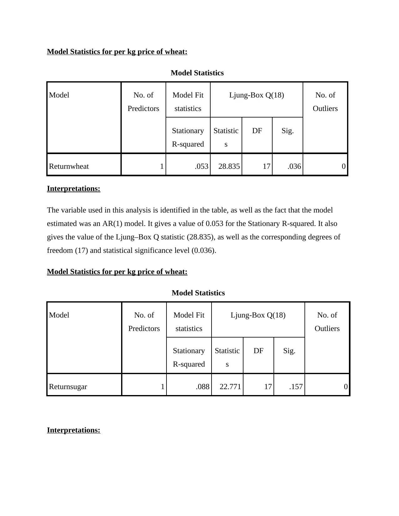
Model Statistics for per kg price of wheat:
Model Statistics
Model No. of
Predictors
Model Fit
statistics
Ljung-Box Q(18) No. of
Outliers
Stationary
R-squared
Statistic
s
DF Sig.
Returnwheat 1 .053 28.835 17 .036 0
Interpretations:
The variable used in this analysis is identified in the table, as well as the fact that the model
estimated was an AR(1) model. It gives a value of 0.053 for the Stationary R-squared. It also
gives the value of the Ljung–Box Q statistic (28.835), as well as the corresponding degrees of
freedom (17) and statistical significance level (0.036).
Model Statistics for per kg price of wheat:
Model Statistics
Model No. of
Predictors
Model Fit
statistics
Ljung-Box Q(18) No. of
Outliers
Stationary
R-squared
Statistic
s
DF Sig.
Returnsugar 1 .088 22.771 17 .157 0
Interpretations:
Model Statistics
Model No. of
Predictors
Model Fit
statistics
Ljung-Box Q(18) No. of
Outliers
Stationary
R-squared
Statistic
s
DF Sig.
Returnwheat 1 .053 28.835 17 .036 0
Interpretations:
The variable used in this analysis is identified in the table, as well as the fact that the model
estimated was an AR(1) model. It gives a value of 0.053 for the Stationary R-squared. It also
gives the value of the Ljung–Box Q statistic (28.835), as well as the corresponding degrees of
freedom (17) and statistical significance level (0.036).
Model Statistics for per kg price of wheat:
Model Statistics
Model No. of
Predictors
Model Fit
statistics
Ljung-Box Q(18) No. of
Outliers
Stationary
R-squared
Statistic
s
DF Sig.
Returnsugar 1 .088 22.771 17 .157 0
Interpretations:
⊘ This is a preview!⊘
Do you want full access?
Subscribe today to unlock all pages.
Trusted by 1+ million students worldwide
1 out of 15
Related Documents


Your All-in-One AI-Powered Toolkit for Academic Success.
+13062052269
info@desklib.com
Available 24*7 on WhatsApp / Email
![[object Object]](/_next/static/media/star-bottom.7253800d.svg)
Unlock your academic potential
Copyright © 2020–2026 A2Z Services. All Rights Reserved. Developed and managed by ZUCOL.