Remote Sensing: Georectification Report - STEM 2001 & 8003 Workshop 2

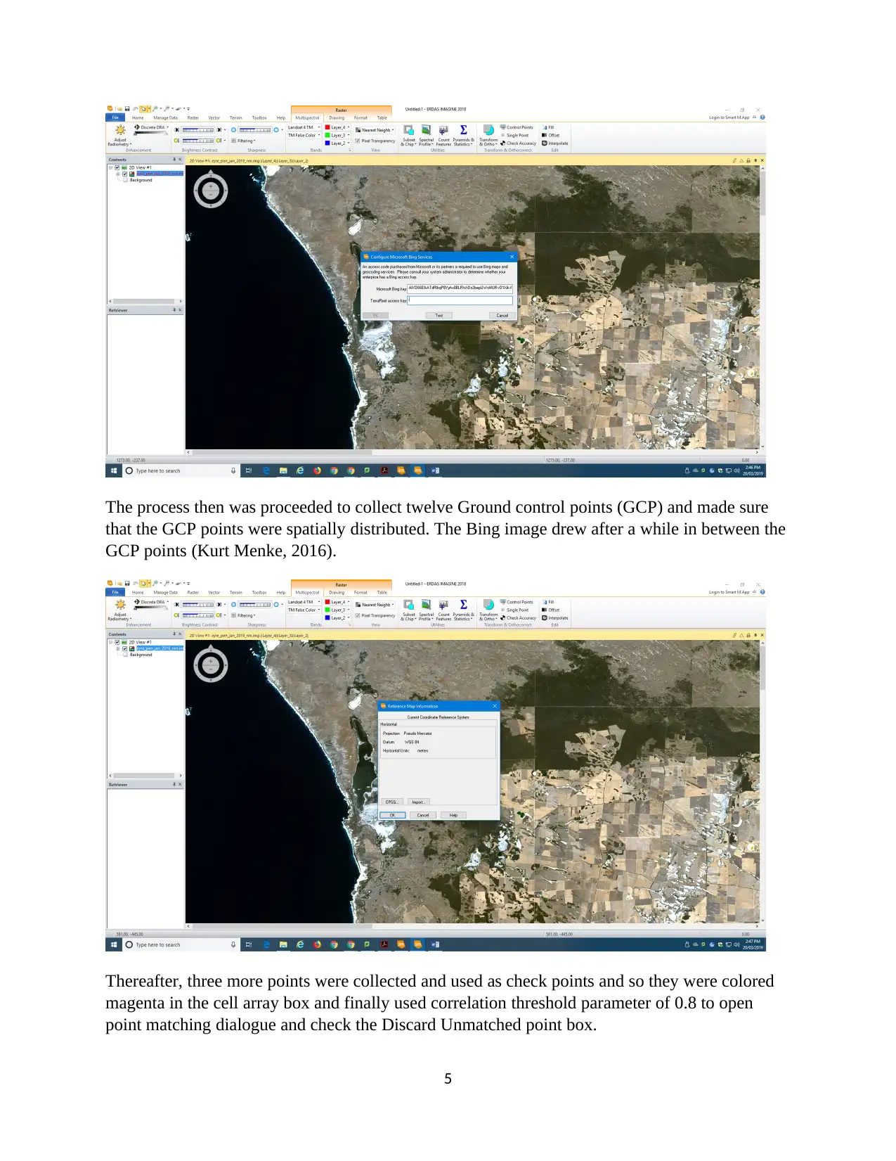
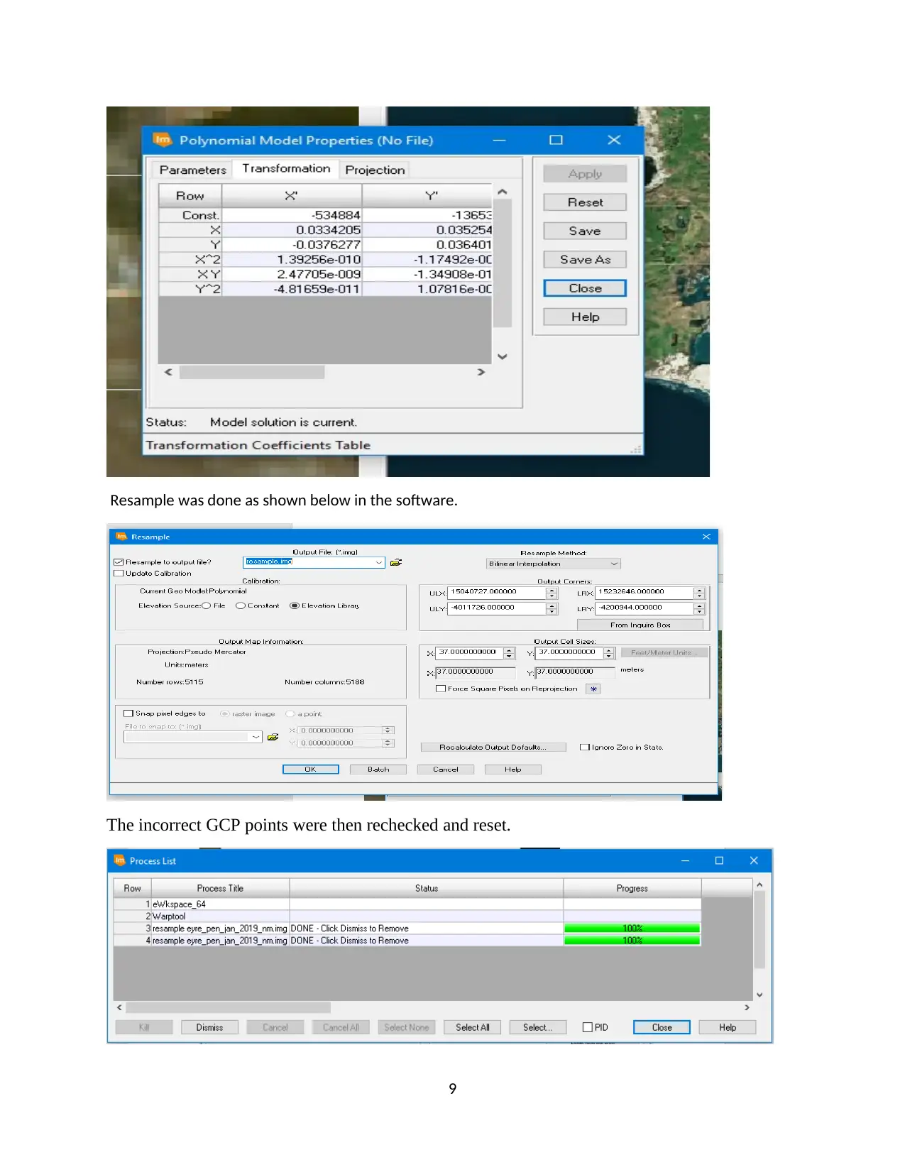
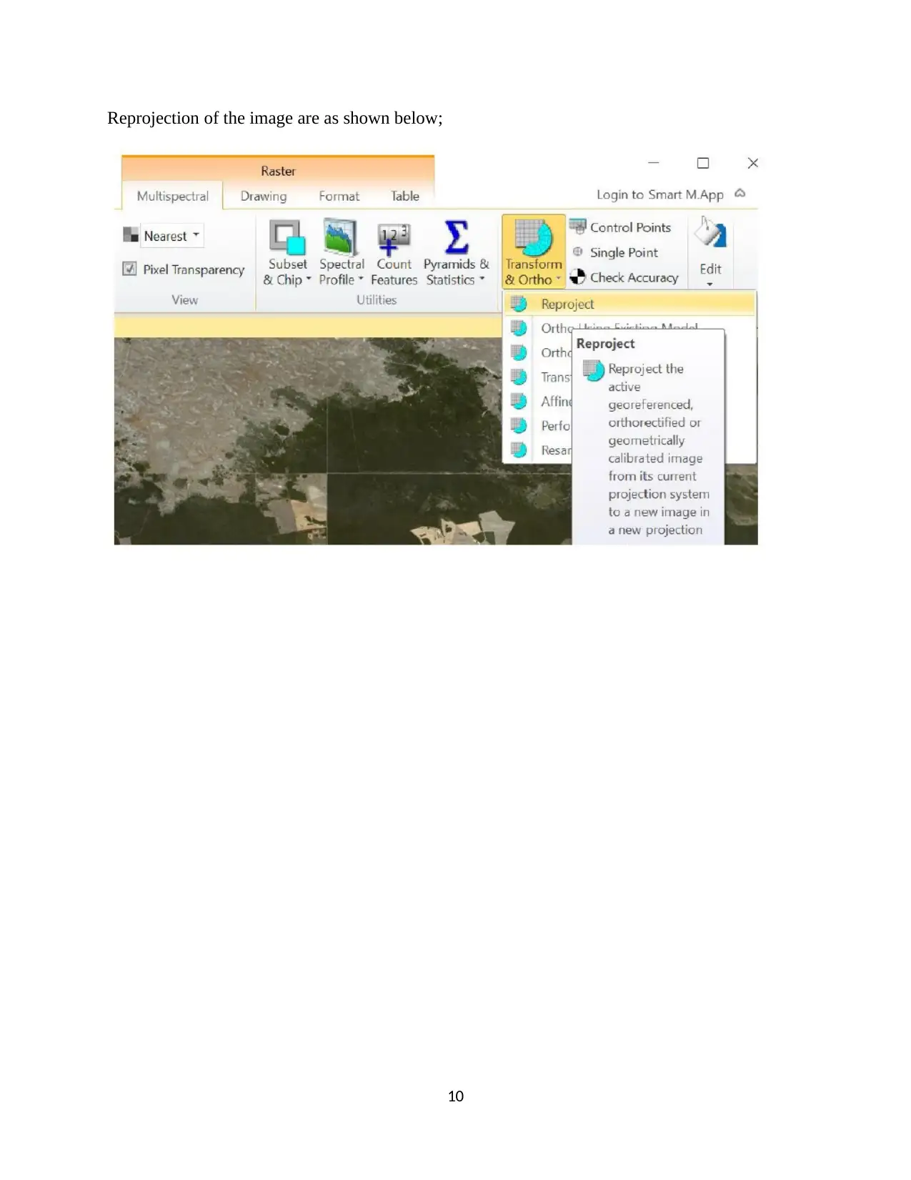
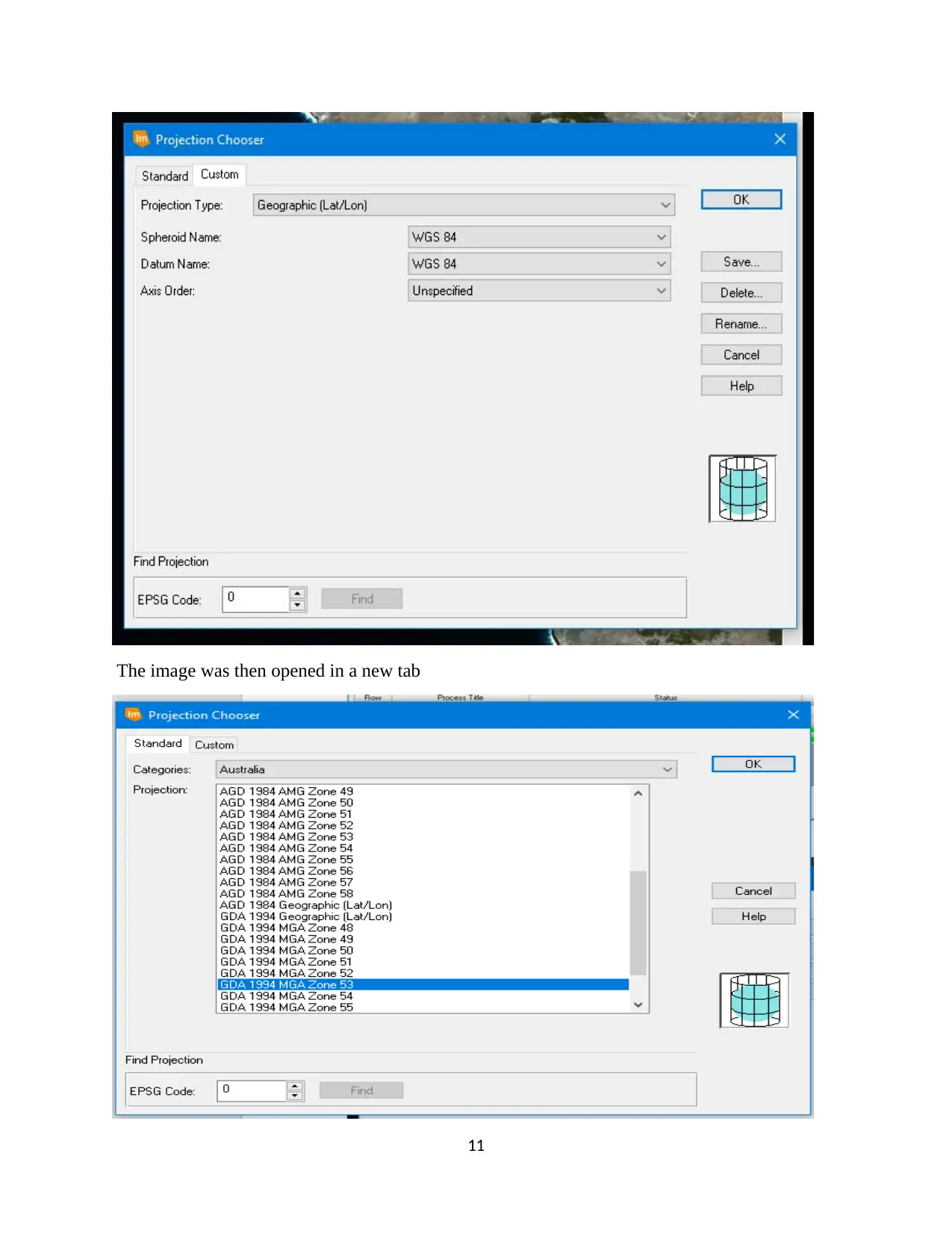
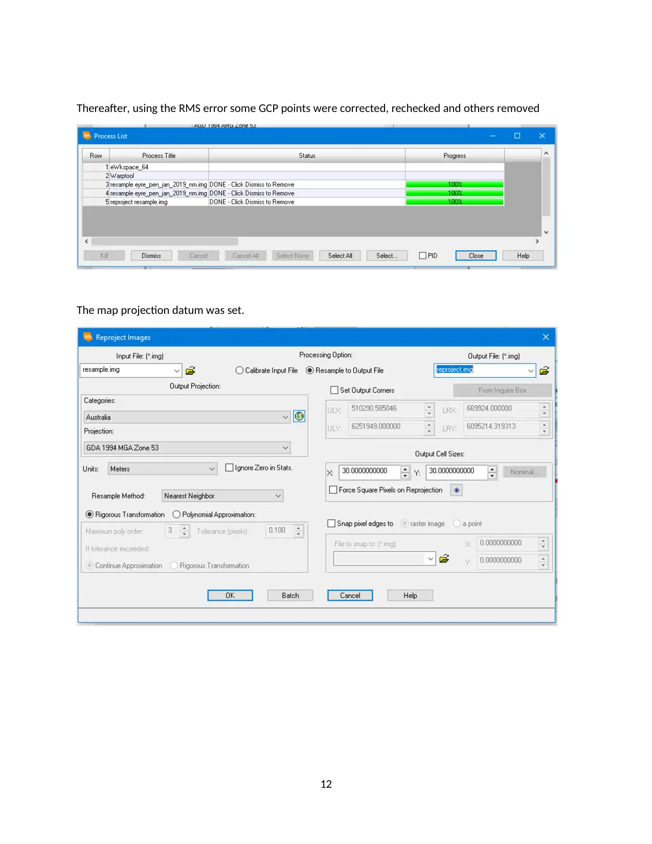
This report details the process of georectifying a satellite image of the Eyre Peninsula using Erdas Imagine software. The study involved opening the image, selecting the Bing Aerial Layer for comparison, collecting and spatially distributing ground control points (GCPs), and calculating the root mean square (RMS) error to assess accuracy. The report outlines the steps of the georectification process, including the use of polynomial transformation, resampling, and reprojection to ensure the image is accurately georeferenced. The results section presents the calculated errors and the identification of features in the reprojected image. The report concludes with a summary emphasizing the accuracy of the georeferencing process and the effectiveness of error reduction techniques, such as the use of RMS error, in achieving spatially accurate maps. Appendix A includes the final images of the Eyre Peninsula.

Geography Report
GEORECTIFICATION
Table of Contents
Objectives………………………………………………………………………….......1
Introduction……………………………………………………………………………1
Material and methods………………………………………………………………….1-13
Results and discussion…………………………………………………………………14-15
Summary………………………………………………………………………………16
Flow chart………………………………………………………………………………17
Reference………………………………………………………………………………18
1

Objectives
The object of this study was to learn on how to use Erdas Imagine and the try to geeorectify a satellite
image of the Eyre Peninsula to enable its use in spatially accurate mapping (Antonio Pratelli, 2011).
Introduction
Erdas imagine is a new tool on the market. It is an image processing application that can be used
to process various data including geospatial, imagery and vector data. The advantage of this tool
over tools of similar is that it can process hyperspectral imagery and LiDAR from various
sensors and also offers 3-dimensional viewing module, that is virtualGIS. In addition, Erdas is a
remote sensing tool (Miljenko Lapaine, 2017).
This surveying tool is available commercially and has been in continued development beginning
1978 by the parent company, Erdas (Gao, 2009). Basically, this tool, Erdas uses pixels for
visualization, manipulation and analysis of aerial and satellite images and various geographical
data. Erdas offers many image processing functions and they include orthorectification, GIS
analysis, production of maps, SAR image processing and 3-dimensional visualization.
Materials and Methods
The study started by opening the Erdas image too and after copying the folder file containing
Eyre Peninsula data and pasted the file into a portable hard drive.
Then the main panel was opened and selected “open raster layer” and thereafter navigated to
where the file was and opened through application (Gustavo Camps, 2011).
2

The image file for rectification was put into the Erdas software
After fitting the image of Eyre Peninsula to frame the group tried to investigate the dataset using
different multispectral band combinations with the aim of examining vegetation, soil, urban
development and many more.
3

After opening transform and ortho-correct group, the Bing Aerail Layer was selected and it
finally opened in a multipoint geometric correction view. The Bing aerial view will eventually
load in the RHS and Australia and then Eyre Peninsula were located. The image of Eyre
Peninsula was then zoomed and compared with the image under georectification (Wilpen L.
Gorr, 2016).
Transform & Ortho-correct group icon was then opened which then opened the multipoint
geometric correction workspace.
4

The process then was proceeded to collect twelve Ground control points (GCP) and made sure
that the GCP points were spatially distributed. The Bing image drew after a while in between the
GCP points (Kurt Menke, 2016).
Thereafter, three more points were collected and used as check points and so they were colored
magenta in the cell array box and finally used correlation threshold parameter of 0.8 to open
point matching dialogue and check the Discard Unmatched point box.
5

The error was then computed and checked the accuracy of our checkpoints. This process was
done by selecting the last GCP checkpoint and see the at the status bar if the check point is
displayed and if it is less than 1 pixel. The map of Australia wa put and the Eyre Peninsula was
zoomed as shown below.
6

Extra GCPS points were collected and errors computed and the Eyre Peninsula was zoomed into
focus
The error should be less than 1 pixel. Thereafter the model properties and transformation tab
were opened which show polynomial coefficients. The coefficients were used to warp original
satellite image to create new georeferenced image and then record the coefficients in the results
section.
7

Finally, the image was re-sampled and applied the mathematical transformation to calculate the
file values for our rectified image.
This was done by clicking the resample icon and opening the dialog window and choosing a
suitable interpolation method and set the output pixel size to 30 meters and finally executed the
output and saved it. It was then checked to see if the Georectification process had created an
image in Pseudo-Mercator WGS84 map projection and datum. After this it was decided to have
the final image in UTM map projection and therefore reprojected the image to UTM using
Geodetic Datum of Australia 1994.
Then the RMS error was calculated as shown below;
8

Resample was done as shown below in the software.
The incorrect GCP points were then rechecked and reset.
9

Reprojection of the image are as shown below;
10

The image was then opened in a new tab
11

Thereafter, using the RMS error some GCP points were corrected, rechecked and others removed
The map projection datum was set.
12

GCP points were checked and collected and the image was under a grey overlay.
The image is ready to save as shown below.
The resulting images and final map of Eyre Peninsula were recorded in the results section (check
final images of Eyre Peninsula in the appendix A).
13

Results and Discussion
Map resolution is usually a function of the latitude, zoom level, and a constant value. This
constant is based on the diameter of the earth (Prasad S. Thenkabail, 2016). Therefore, at a
particular latitude we can calculate the scale using the equation;
Map resolution = 156543.04 meters per pixel *cos (latitude) / (2^zoomlevel)
The spatial resolution of the Binge is better than the one of the unreferenced satellite imageries.
From the results that were obtained from the study the root mean squire error and the total error
were calculated as shown from the table.
The control point error for X was 0.2960 and for Y was 0.3874 and the total error was calculated
as 0.4875
The features that can be found on the final reprojected image at four coordinates of landscape
feature 556927 6202906 578273 6156267 607256 6123421 539848 6158909 include woodland,
shrubs and grass.
When the study was being done it was noticed that the GCPs generally did not fall perfectly on
the trend line and so the distance of each GCP from the regression was measured by the root
mean error, RMS error. In the study the total RMS error was 0.4875 which when converted to
ground distance in meters, it means that the error between the GCP and the actual ground was
0.4875 meters (Daniel McInerney, 2014).
Rectifying or warping basically creates a new raster dataset that is georeferenced using the map
coordinates and the spatial reference. Warping can be done using any of the three methods;
rotation, scaling and translation (RST), polynomial and triangulation. And in this study, the most
suitable method to be used is polynomial in which the polynomial coefficients from the 1st to nth
degree and since the GCP points were for spatially accurate map of Eyre Peninsula. In
polynomial warping, desired polynomial Degree is taken into account and the degree available is
dependent on the number of ground collecting points available, where #GCPs > (degree + 1)2
(National Research Council, Division on Earth and Life Studies, Board on Earth Sciences and
Resources, Committee on Seismology and Geodynamics, Committee on the National
Requirements for Precision Geodetic Infrastructure, 2010).
14

When rectifying the GCPs with large RMS errors, the points should be rechecked because they
may be incorrectly located. The objective is to arrive at an overall RMS error of less than 1 pixel
and in our study the overall RMS error was 0.4875 and so it met the objective. Errors caused by
incorrectly located GCPs are minimized by rechecking and relocating them.
15

Summary
In brief, this process of georeferencing and georectification using Erdas equipment is very
accurate as can be seen from this study. Rectification of GCP points using various methods of
error reduction such Root Mean Squire error can be used to correct out-of-location points. The
Erdas software also gives the surveyor quality and well depicted images.
Appendix A
Final Image A;
Image B
16

Flow Chart
References
Antonio Pratelli, C. A. B., 2011. Urban Transport XVII: Urban Transport and the Environment
in the 21st Century. 1 ed. London: WIT Press.
17
Eye Peninsula Bing Map
Georectification
Process
Ground Control Points
Resampling Reprojection Final image
Polynomial
Order

Daniel McInerney, P. K., 2014. Open Source Geospatial Tools: Applications in Earth
Observation. 2 ed. London: Springer.
Gao, J., 2009. Digital Analysis of Remotely Sensed Imagery. 1 ed. London: McGraw Hill
Professional.
Gustavo Camps, G. C.-V., 2011. Remote Sensing Image Processing. 1 ed. New York: Morgan &
Claypool Publishers.
Kurt Menke, G. D. R. S. J. G. D. L. P. D. J. V. H. G., 2016. Mastering QGIS. 2 ed. Birmingham:
Packt Publishing Ltd.
Miljenko Lapaine, E. L. U., 2017. Choosing a Map Projection. 1 ed. New York: Springer.
National Research Council, Division on Earth and Life Studies, Board on Earth Sciences and
Resources, Committee on Seismology and Geodynamics, Committee on the National
Requirements for Precision Geodetic Infrastructure, 2010. Precise Geodetic Infrastructure:
National Requirements for a Shared Resource. Washington DC: National Academies Press.
Prasad S. Thenkabail, J. G. L., 2016. Hyperspectral Remote Sensing of Vegetation. 2 ed. London:
CRC Press.
Wilpen L. Gorr, K. S. K., 2016. GIS Tutorial One, Volume 1. 6 ed. Philadelphia: Esri Press.
18