Analysis of Dwelling Type, Bedrooms, and Suburb on Rental Costs

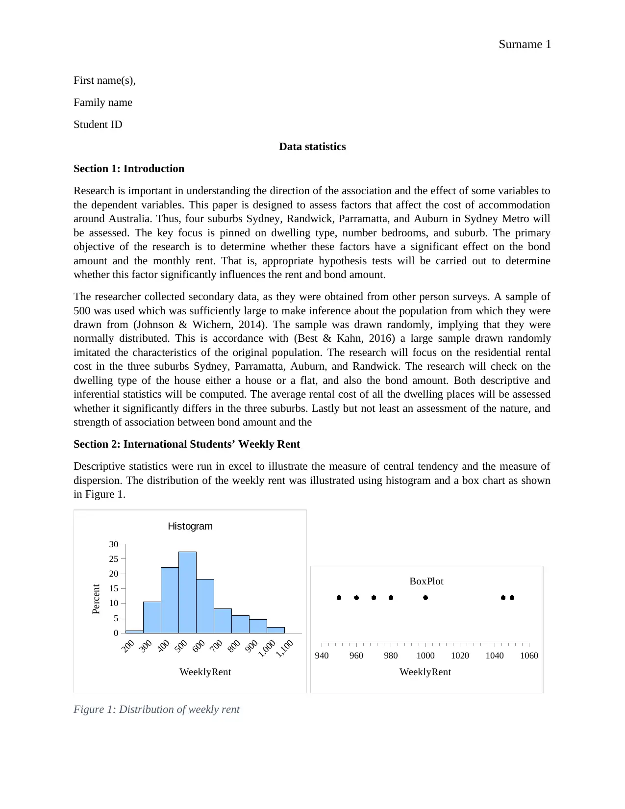
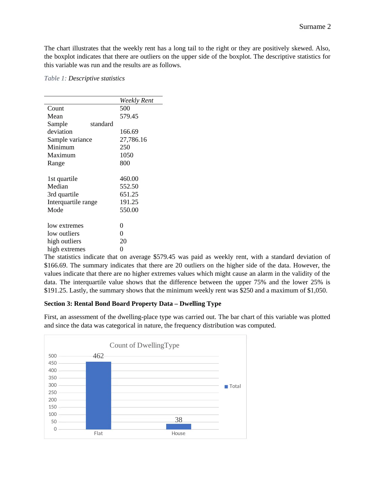
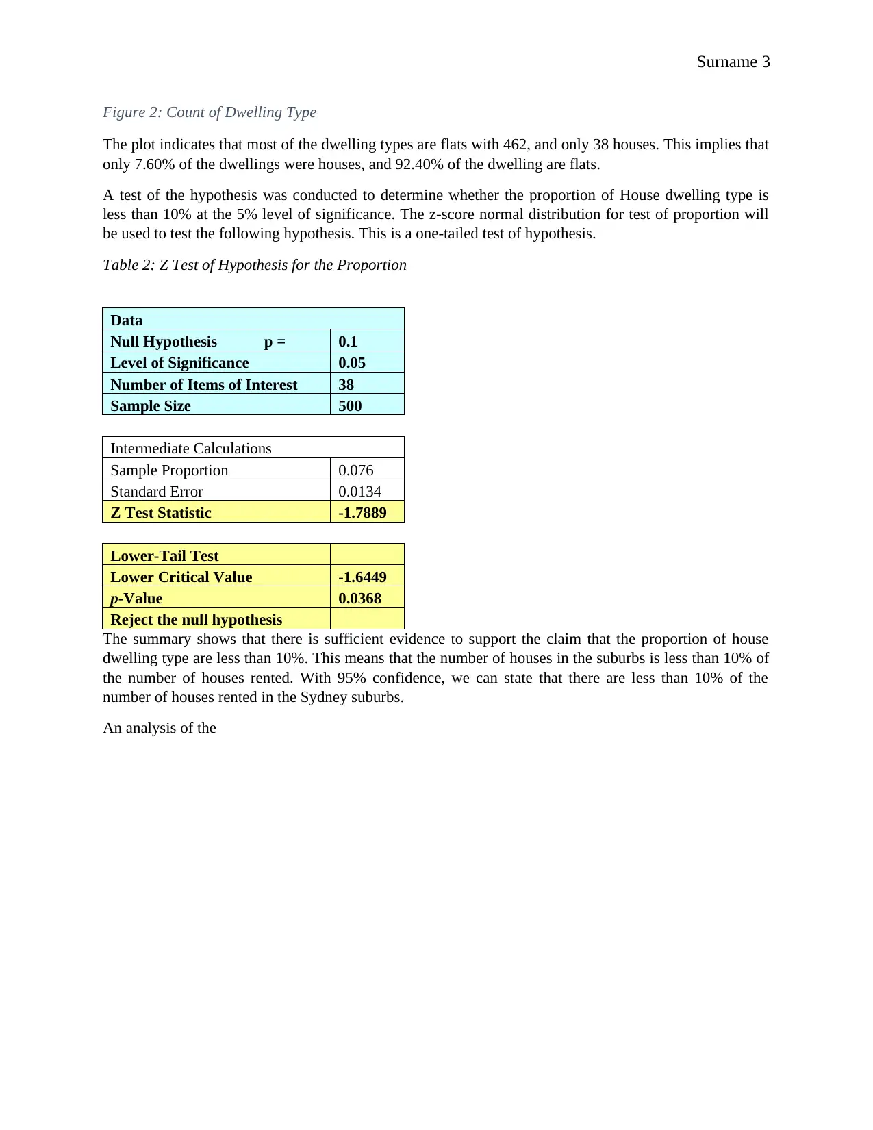
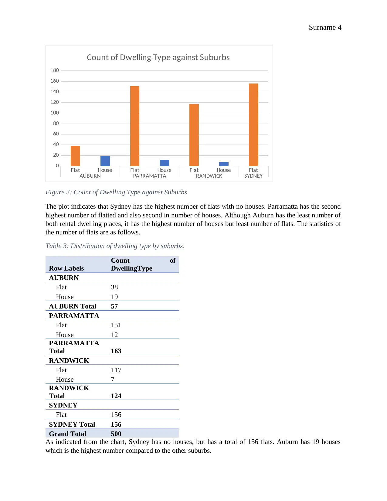
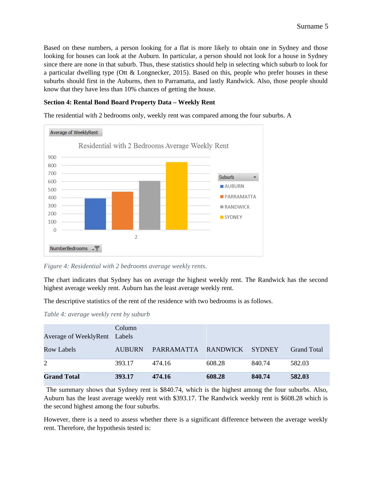
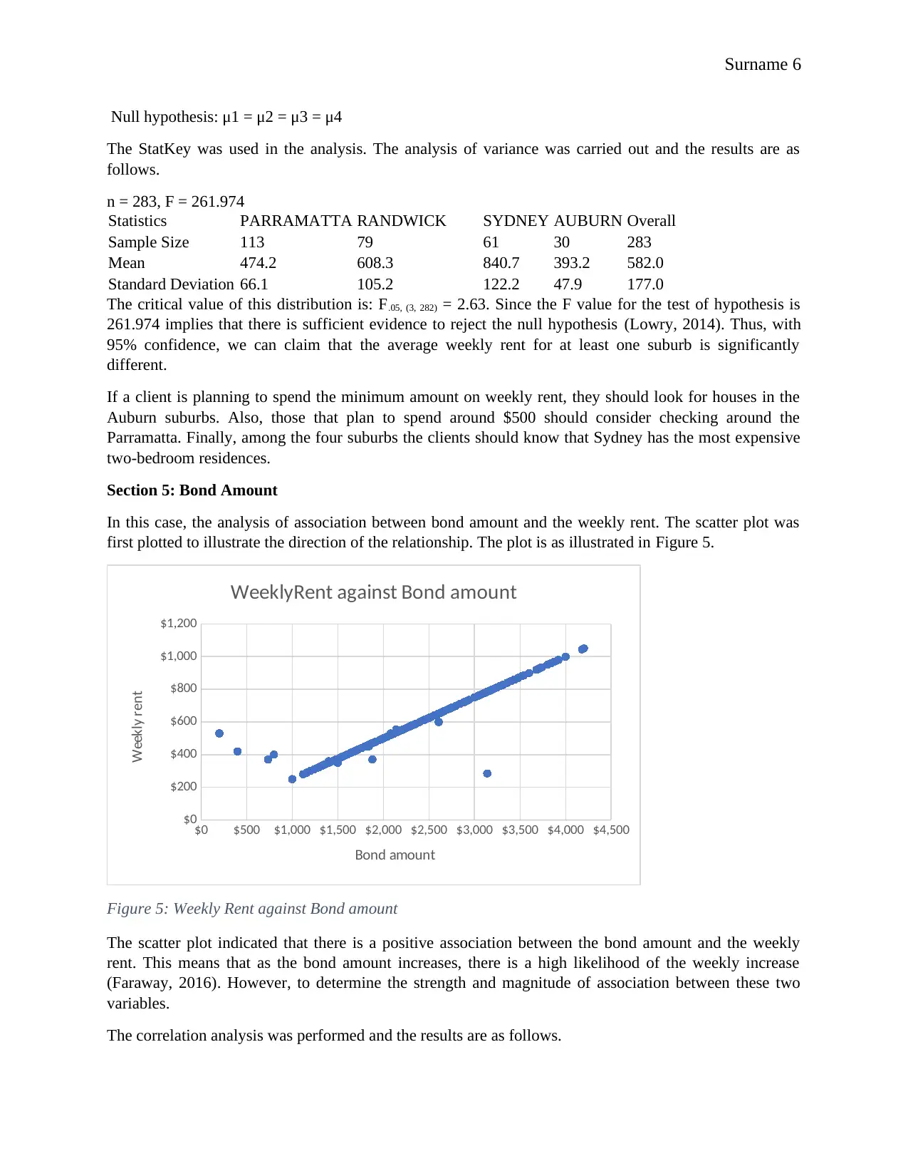
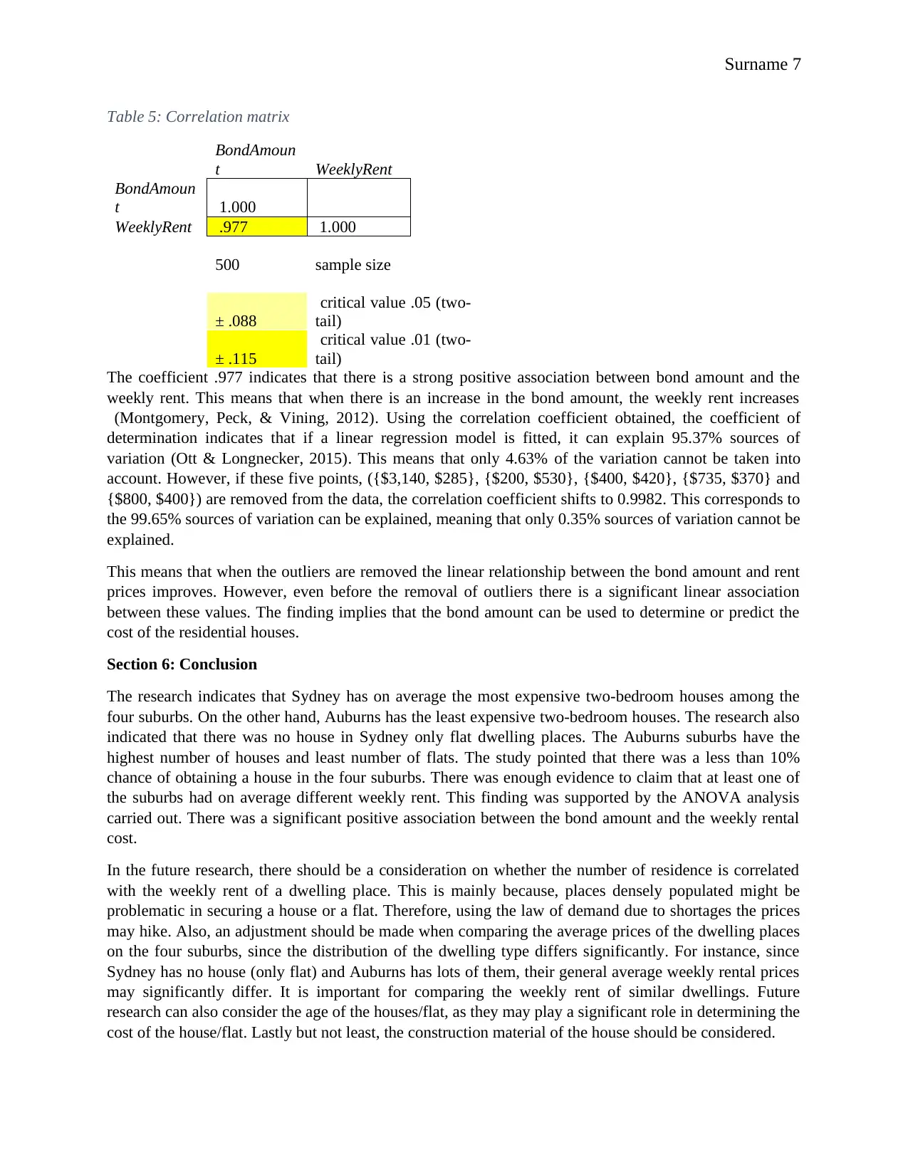
This report presents a statistical analysis of factors affecting rental costs in four Sydney suburbs: Sydney, Randwick, Parramatta, and Auburn. The study investigates the influence of dwelling type (house vs. flat), number of bedrooms, and suburb on bond amounts and monthly rent. Using secondary data from a sample of 500, the research employs descriptive and inferential statistics, including hypothesis testing and correlation analysis. Key findings reveal that Sydney has the highest average weekly rent for two-bedroom residences, while Auburn has the lowest. The report demonstrates a significant positive association between bond amount and weekly rent. The analysis also examines the distribution of dwelling types across suburbs, finding that flats are more prevalent than houses. The report concludes with recommendations for future research, including considerations for the number of residences, dwelling type distribution, age, and construction materials of the properties. The study aims to provide valuable insights into the Australian rental market.

Surname 1
First name(s),
Family name
Student ID
Data statistics
Section 1: Introduction
Research is important in understanding the direction of the association and the effect of some variables to
the dependent variables. This paper is designed to assess factors that affect the cost of accommodation
around Australia. Thus, four suburbs Sydney, Randwick, Parramatta, and Auburn in Sydney Metro will
be assessed. The key focus is pinned on dwelling type, number bedrooms, and suburb. The primary
objective of the research is to determine whether these factors have a significant effect on the bond
amount and the monthly rent. That is, appropriate hypothesis tests will be carried out to determine
whether this factor significantly influences the rent and bond amount.
The researcher collected secondary data, as they were obtained from other person surveys. A sample of
500 was used which was sufficiently large to make inference about the population from which they were
drawn from (Johnson & Wichern, 2014). The sample was drawn randomly, implying that they were
normally distributed. This is accordance with (Best & Kahn, 2016) a large sample drawn randomly
imitated the characteristics of the original population. The research will focus on the residential rental
cost in the three suburbs Sydney, Parramatta, Auburn, and Randwick. The research will check on the
dwelling type of the house either a house or a flat, and also the bond amount. Both descriptive and
inferential statistics will be computed. The average rental cost of all the dwelling places will be assessed
whether it significantly differs in the three suburbs. Lastly but not least an assessment of the nature, and
strength of association between bond amount and the
Section 2: International Students’ Weekly Rent
Descriptive statistics were run in excel to illustrate the measure of central tendency and the measure of
dispersion. The distribution of the weekly rent was illustrated using histogram and a box chart as shown
in Figure 1.
200
300
400
500
600
700
800
900
1,000
1,100
0
5
10
15
20
25
30
Histogram
WeeklyRent
Percent
940 960 980 1000 1020 1040 1060
BoxPlot
WeeklyRent
Figure 1: Distribution of weekly rent

Surname 2
The chart illustrates that the weekly rent has a long tail to the right or they are positively skewed. Also,
the boxplot indicates that there are outliers on the upper side of the boxplot. The descriptive statistics for
this variable was run and the results are as follows.
Table 1: Descriptive statistics
Weekly Rent
Count 500
Mean 579.45
Sample standard
deviation 166.69
Sample variance 27,786.16
Minimum 250
Maximum 1050
Range 800
1st quartile 460.00
Median 552.50
3rd quartile 651.25
Interquartile range 191.25
Mode 550.00
low extremes 0
low outliers 0
high outliers 20
high extremes 0
The statistics indicate that on average $579.45 was paid as weekly rent, with a standard deviation of
$166.69. The summary indicates that there are 20 outliers on the higher side of the data. However, the
values indicate that there are no higher extremes values which might cause an alarm in the validity of the
data. The interquartile value shows that the difference between the upper 75% and the lower 25% is
$191.25. Lastly, the summary shows that the minimum weekly rent was $250 and a maximum of $1,050.
Section 3: Rental Bond Board Property Data – Dwelling Type
First, an assessment of the dwelling-place type was carried out. The bar chart of this variable was plotted
and since the data was categorical in nature, the frequency distribution was computed.
Flat House
0
50
100
150
200
250
300
350
400
450
500 462
38
Count of DwellingType
Total

Surname 3
Figure 2: Count of Dwelling Type
The plot indicates that most of the dwelling types are flats with 462, and only 38 houses. This implies that
only 7.60% of the dwellings were houses, and 92.40% of the dwelling are flats.
A test of the hypothesis was conducted to determine whether the proportion of House dwelling type is
less than 10% at the 5% level of significance. The z-score normal distribution for test of proportion will
be used to test the following hypothesis. This is a one-tailed test of hypothesis.
Table 2: Z Test of Hypothesis for the Proportion
Data
Null Hypothesis p = 0.1
Level of Significance 0.05
Number of Items of Interest 38
Sample Size 500
Intermediate Calculations
Sample Proportion 0.076
Standard Error 0.0134
Z Test Statistic -1.7889
Lower-Tail Test
Lower Critical Value -1.6449
p-Value 0.0368
Reject the null hypothesis
The summary shows that there is sufficient evidence to support the claim that the proportion of house
dwelling type are less than 10%. This means that the number of houses in the suburbs is less than 10% of
the number of houses rented. With 95% confidence, we can state that there are less than 10% of the
number of houses rented in the Sydney suburbs.
An analysis of the

Surname 4
Flat House Flat House Flat House Flat
AUBURN PARRAMATTA RANDWICK SYDNEY
0
20
40
60
80
100
120
140
160
180
Count of Dwelling Type against Suburbs
Figure 3: Count of Dwelling Type against Suburbs
The plot indicates that Sydney has the highest number of flats with no houses. Parramatta has the second
highest number of flatted and also second in number of houses. Although Auburn has the least number of
both rental dwelling places, it has the highest number of houses but least number of flats. The statistics of
the number of flats are as follows.
Table 3: Distribution of dwelling type by suburbs.
Row Labels
Count of
DwellingType
AUBURN
Flat 38
House 19
AUBURN Total 57
PARRAMATTA
Flat 151
House 12
PARRAMATTA
Total 163
RANDWICK
Flat 117
House 7
RANDWICK
Total 124
SYDNEY
Flat 156
SYDNEY Total 156
Grand Total 500
As indicated from the chart, Sydney has no houses, but has a total of 156 flats. Auburn has 19 houses
which is the highest number compared to the other suburbs.

Surname 5
Based on these numbers, a person looking for a flat is more likely to obtain one in Sydney and those
looking for houses can look at the Auburn. In particular, a person should not look for a house in Sydney
since there are none in that suburb. Thus, these statistics should help in selecting which suburb to look for
a particular dwelling type (Ott & Longnecker, 2015). Based on this, people who prefer houses in these
suburbs should first in the Auburns, then to Parramatta, and lastly Randwick. Also, those people should
know that they have less than 10% chances of getting the house.
Section 4: Rental Bond Board Property Data – Weekly Rent
The residential with 2 bedrooms only, weekly rent was compared among the four suburbs. A
Figure 4: Residential with 2 bedrooms average weekly rents.
The chart indicates that Sydney has on average the highest weekly rent. The Randwick has the second
highest average weekly rent. Auburn has the least average weekly rent.
The descriptive statistics of the rent of the residence with two bedrooms is as follows.
Table 4: average weekly rent by suburb
Average of WeeklyRent
Column
Labels
Row Labels AUBURN PARRAMATTA RANDWICK SYDNEY Grand Total
2 393.17 474.16 608.28 840.74 582.03
Grand Total 393.17 474.16 608.28 840.74 582.03
The summary shows that Sydney rent is $840.74, which is the highest among the four suburbs. Also,
Auburn has the least average weekly rent with $393.17. The Randwick weekly rent is $608.28 which is
the second highest among the four suburbs.
However, there is a need to assess whether there is a significant difference between the average weekly
rent. Therefore, the hypothesis tested is:

Surname 6
Null hypothesis: μ1 = μ2 = μ3 = μ4
The StatKey was used in the analysis. The analysis of variance was carried out and the results are as
follows.
n = 283, F = 261.974
Statistics PARRAMATTA RANDWICK SYDNEY AUBURN Overall
Sample Size 113 79 61 30 283
Mean 474.2 608.3 840.7 393.2 582.0
Standard Deviation 66.1 105.2 122.2 47.9 177.0
The critical value of this distribution is: F.05, (3, 282) = 2.63. Since the F value for the test of hypothesis is
261.974 implies that there is sufficient evidence to reject the null hypothesis (Lowry, 2014). Thus, with
95% confidence, we can claim that the average weekly rent for at least one suburb is significantly
different.
If a client is planning to spend the minimum amount on weekly rent, they should look for houses in the
Auburn suburbs. Also, those that plan to spend around $500 should consider checking around the
Parramatta. Finally, among the four suburbs the clients should know that Sydney has the most expensive
two-bedroom residences.
Section 5: Bond Amount
In this case, the analysis of association between bond amount and the weekly rent. The scatter plot was
first plotted to illustrate the direction of the relationship. The plot is as illustrated in Figure 5.
$0 $500 $1,000 $1,500 $2,000 $2,500 $3,000 $3,500 $4,000 $4,500
$0
$200
$400
$600
$800
$1,000
$1,200
WeeklyRent against Bond amount
Bond amount
Weekly rent
Figure 5: Weekly Rent against Bond amount
The scatter plot indicated that there is a positive association between the bond amount and the weekly
rent. This means that as the bond amount increases, there is a high likelihood of the weekly increase
(Faraway, 2016). However, to determine the strength and magnitude of association between these two
variables.
The correlation analysis was performed and the results are as follows.

Surname 7
Table 5: Correlation matrix
BondAmoun
t WeeklyRent
BondAmoun
t 1.000
WeeklyRent .977 1.000
500 sample size
± .088
critical value .05 (two-
tail)
± .115
critical value .01 (two-
tail)
The coefficient .977 indicates that there is a strong positive association between bond amount and the
weekly rent. This means that when there is an increase in the bond amount, the weekly rent increases
(Montgomery, Peck, & Vining, 2012). Using the correlation coefficient obtained, the coefficient of
determination indicates that if a linear regression model is fitted, it can explain 95.37% sources of
variation (Ott & Longnecker, 2015). This means that only 4.63% of the variation cannot be taken into
account. However, if these five points, ({$3,140, $285}, {$200, $530}, {$400, $420}, {$735, $370} and
{$800, $400}) are removed from the data, the correlation coefficient shifts to 0.9982. This corresponds to
the 99.65% sources of variation can be explained, meaning that only 0.35% sources of variation cannot be
explained.
This means that when the outliers are removed the linear relationship between the bond amount and rent
prices improves. However, even before the removal of outliers there is a significant linear association
between these values. The finding implies that the bond amount can be used to determine or predict the
cost of the residential houses.
Section 6: Conclusion
The research indicates that Sydney has on average the most expensive two-bedroom houses among the
four suburbs. On the other hand, Auburns has the least expensive two-bedroom houses. The research also
indicated that there was no house in Sydney only flat dwelling places. The Auburns suburbs have the
highest number of houses and least number of flats. The study pointed that there was a less than 10%
chance of obtaining a house in the four suburbs. There was enough evidence to claim that at least one of
the suburbs had on average different weekly rent. This finding was supported by the ANOVA analysis
carried out. There was a significant positive association between the bond amount and the weekly rental
cost.
In the future research, there should be a consideration on whether the number of residence is correlated
with the weekly rent of a dwelling place. This is mainly because, places densely populated might be
problematic in securing a house or a flat. Therefore, using the law of demand due to shortages the prices
may hike. Also, an adjustment should be made when comparing the average prices of the dwelling places
on the four suburbs, since the distribution of the dwelling type differs significantly. For instance, since
Sydney has no house (only flat) and Auburns has lots of them, their general average weekly rental prices
may significantly differ. It is important for comparing the weekly rent of similar dwellings. Future
research can also consider the age of the houses/flat, as they may play a significant role in determining the
cost of the house/flat. Lastly but not least, the construction material of the house should be considered.

Surname 8
References
Best, J. W., & Kahn, J. V. (2016). Research in education. India: Pearson Education.
Faraway, J. J. (2016, March 23). Extending the linear model with R: generalized linear, mixed effects and
nonparametric regression models. 124. CRC press.
Johnson, R. A., & Wichern, D. W. (2014). Applied multivariate statistical analysis (Vol. 4). New Jersey:
Prentice-Hall.
Lowry, R. (2014). Concepts and applications of inferential statistics.
Montgomery, D. C., Peck, E. A., & Vining, G. G. (2012). Introduction to linear regression analysis. 821.
John Wiley & Sons.
Ott, R. L., & Longnecker, M. T. (2015). An introduction to statistical methods and data analysis. Nelson
Education.