HI6007: Statistics and Research Methods Group Assignment T1 2019

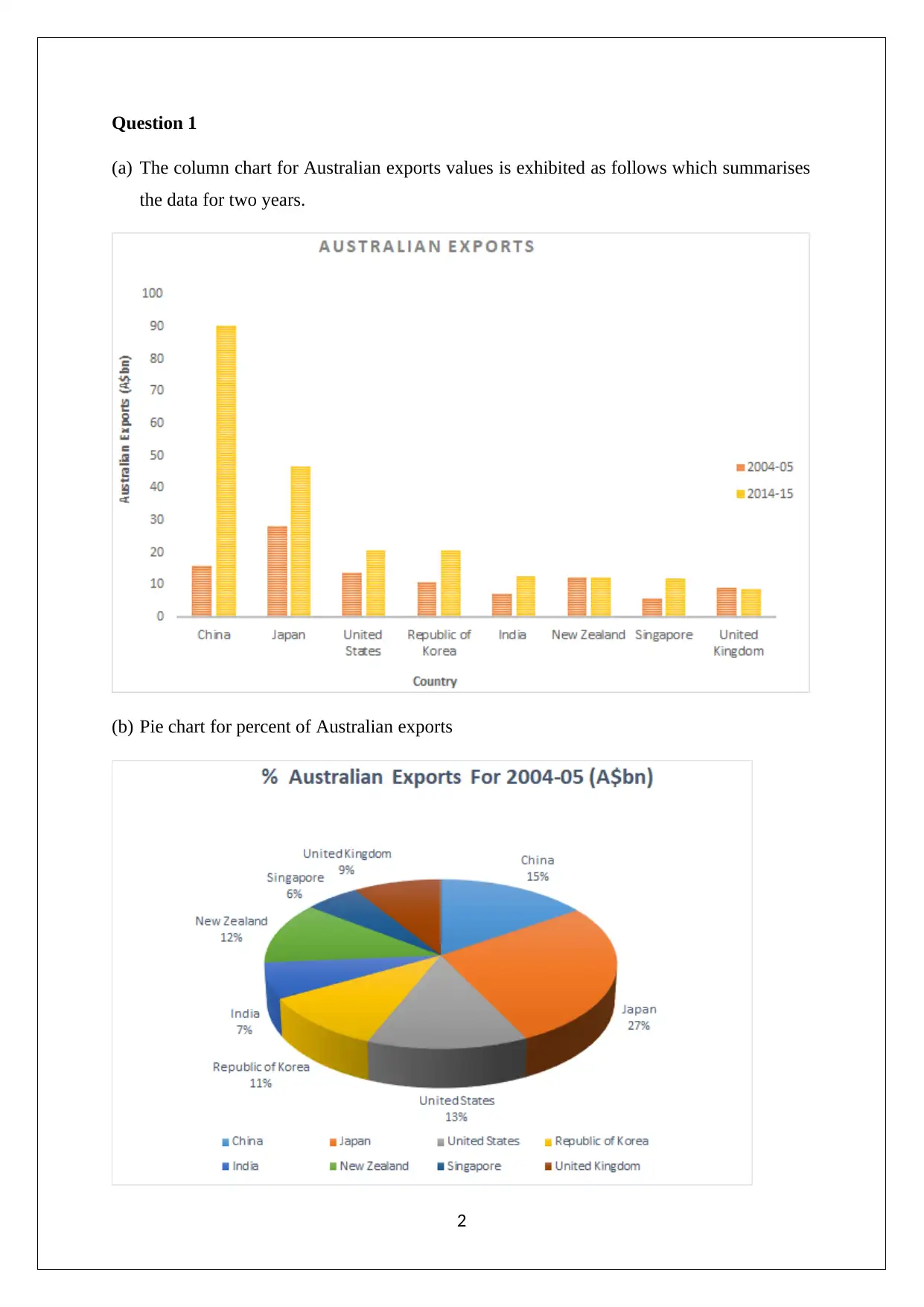
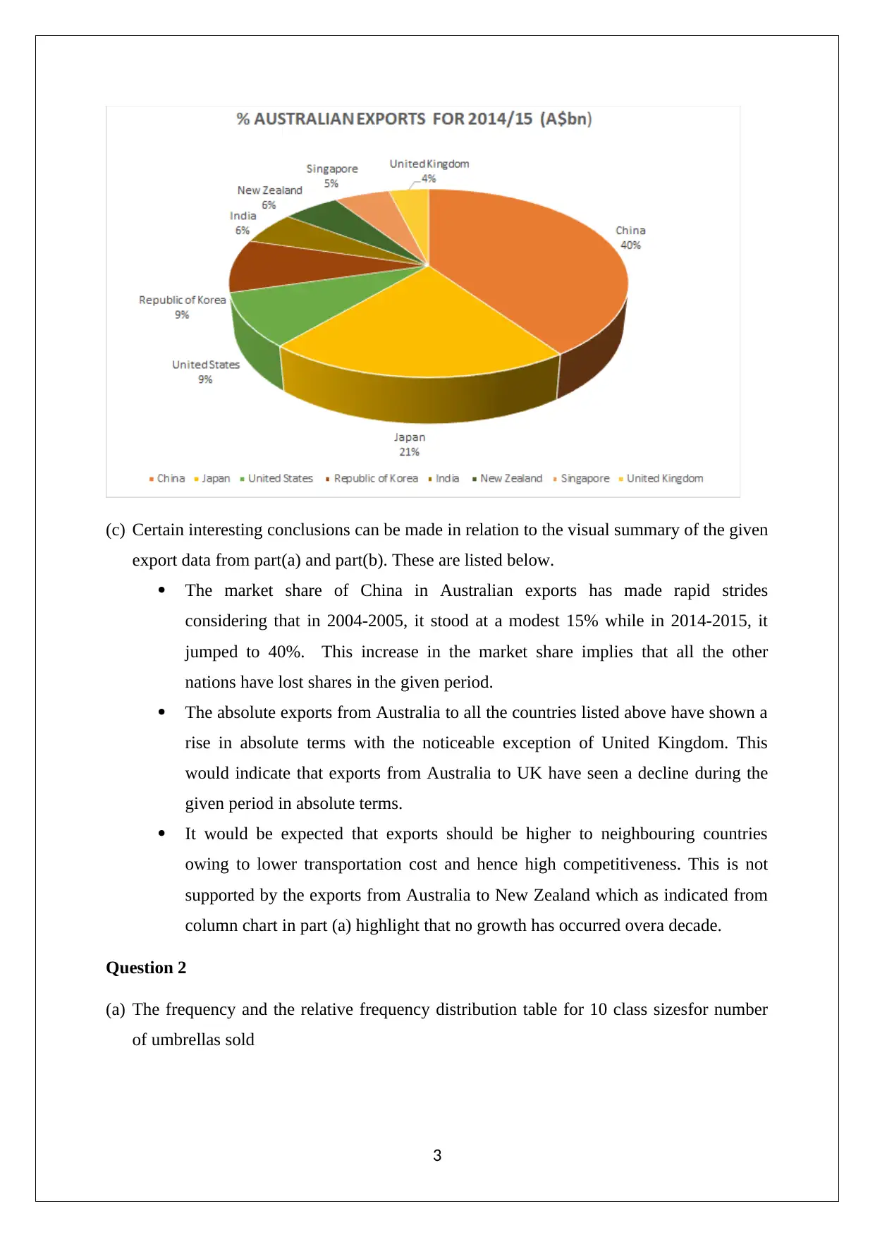
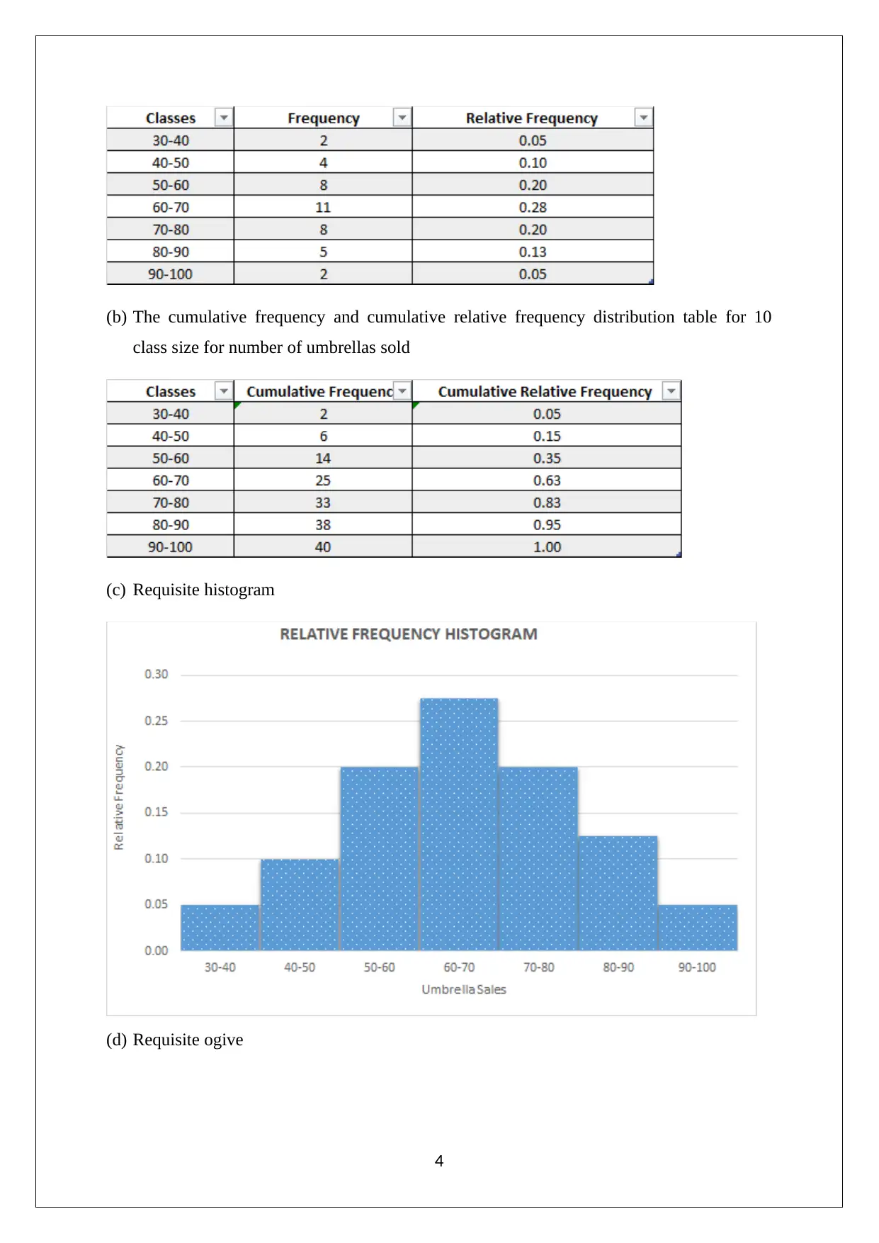
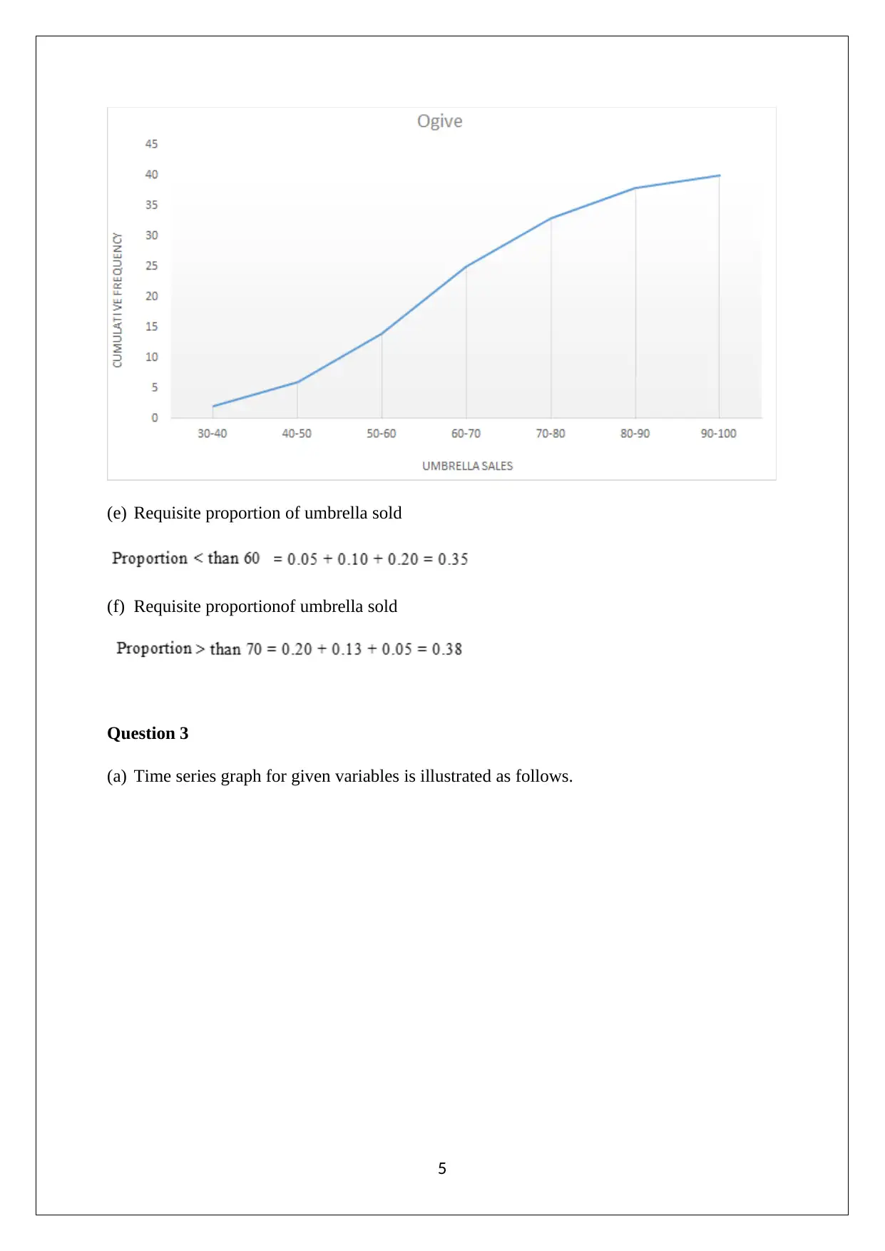
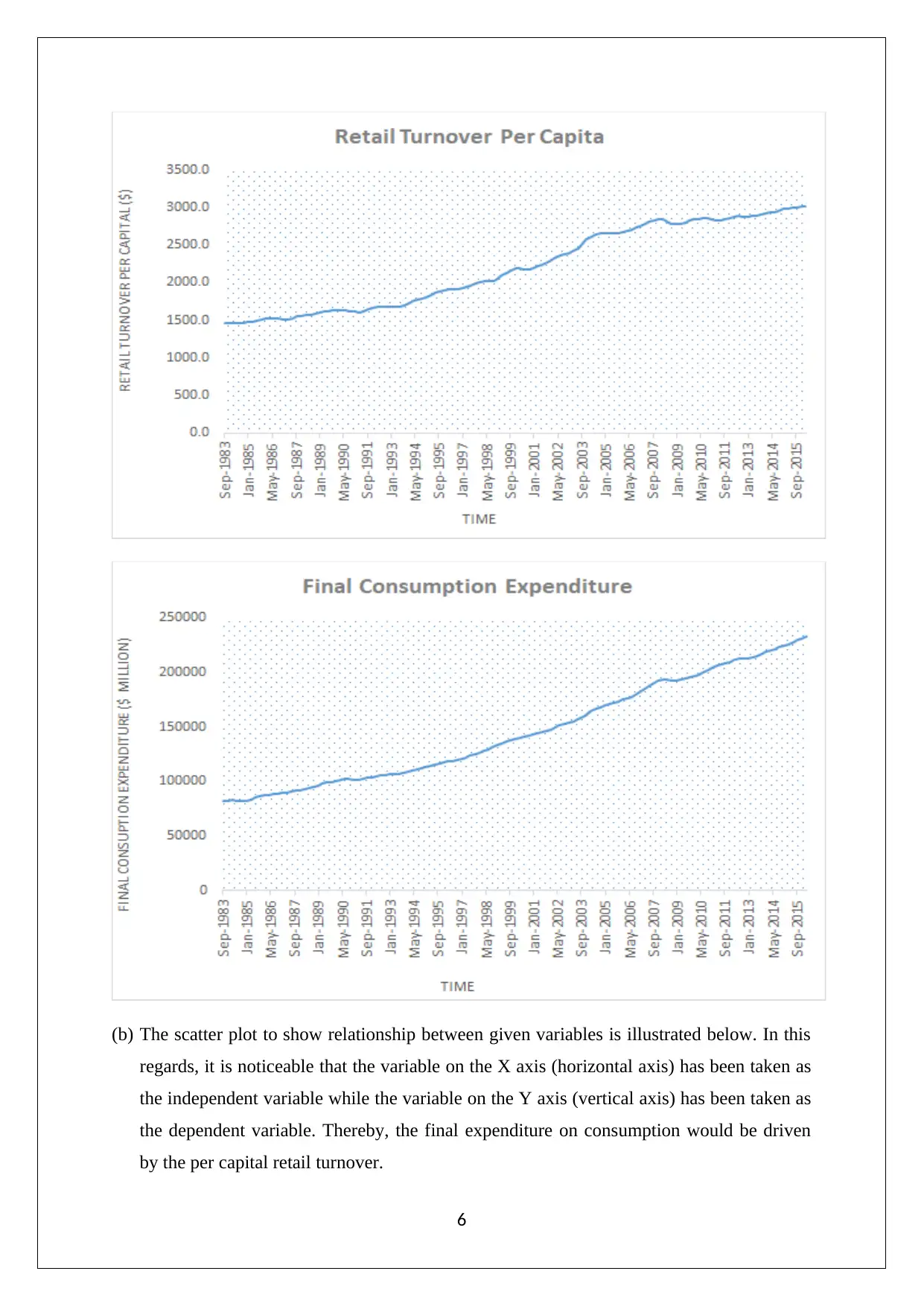
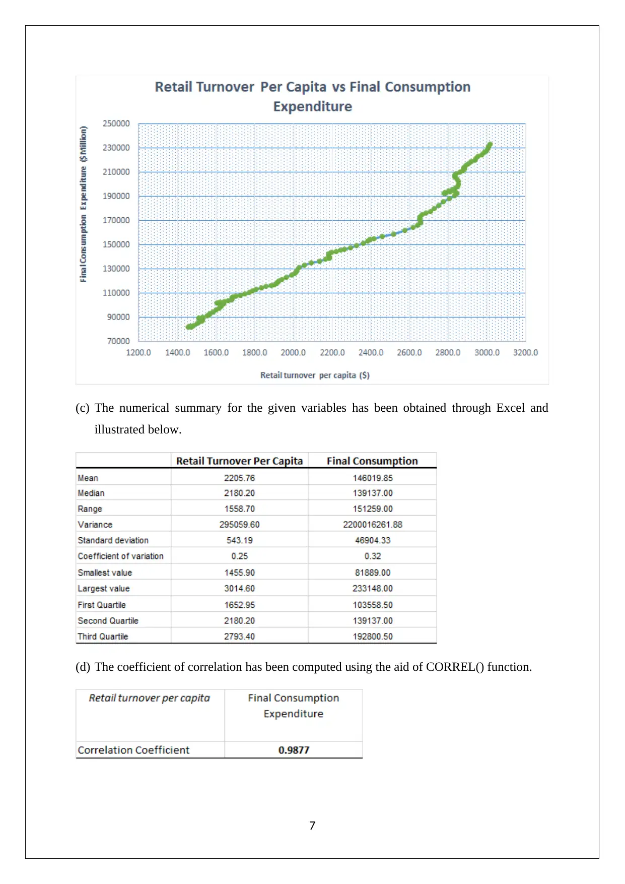
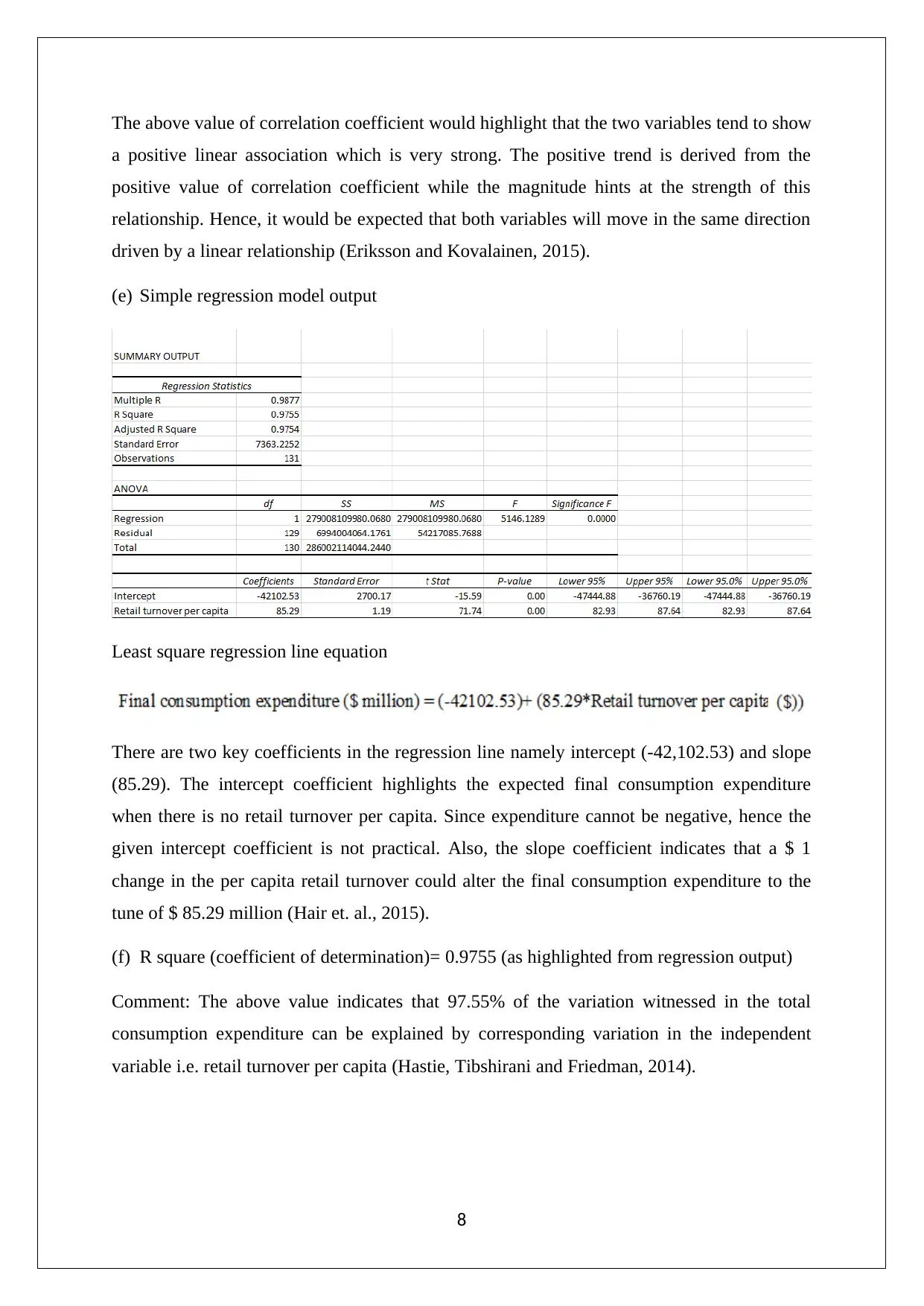
This assignment solution for the Statistics and Research Methods for Business Decision Making course (HI6007) covers various statistical concepts and their application in business contexts. The solution includes analysis of Australian export data using column and pie charts, drawing conclusions about market share changes and export trends. It also presents frequency distributions, histograms, and ogives related to umbrella sales data. Furthermore, the assignment delves into time series analysis and regression modeling, exploring the relationship between retail turnover per capita and final consumption expenditure. It provides a numerical summary, correlation analysis, regression model output, and hypothesis testing to determine the significance of the relationship. The document also includes references to support the analysis and findings.

Statistics and Research Methods for Business Decision Making
[Type the document subtitle]
STUDENT ID:
[Pick the date]

Question 1
(a) The column chart for Australian exports values is exhibited as follows which summarises
the data for two years.
(b) Pie chart for percent of Australian exports
2

(c) Certain interesting conclusions can be made in relation to the visual summary of the given
export data from part(a) and part(b). These are listed below.
 The market share of China in Australian exports has made rapid strides
considering that in 2004-2005, it stood at a modest 15% while in 2014-2015, it
jumped to 40%. This increase in the market share implies that all the other
nations have lost shares in the given period.
 The absolute exports from Australia to all the countries listed above have shown a
rise in absolute terms with the noticeable exception of United Kingdom. This
would indicate that exports from Australia to UK have seen a decline during the
given period in absolute terms.
 It would be expected that exports should be higher to neighbouring countries
owing to lower transportation cost and hence high competitiveness. This is not
supported by the exports from Australia to New Zealand which as indicated from
column chart in part (a) highlight that no growth has occurred overa decade.
Question 2
(a) The frequency and the relative frequency distribution table for 10 class sizesfor number
of umbrellas sold
3

(b) The cumulative frequency and cumulative relative frequency distribution table for 10
class size for number of umbrellas sold
(c) Requisite histogram
(d) Requisite ogive
4

(e) Requisite proportion of umbrella sold
(f) Requisite proportionof umbrella sold
Question 3
(a) Time series graph for given variables is illustrated as follows.
5

(b) The scatter plot to show relationship between given variables is illustrated below. In this
regards, it is noticeable that the variable on the X axis (horizontal axis) has been taken as
the independent variable while the variable on the Y axis (vertical axis) has been taken as
the dependent variable. Thereby, the final expenditure on consumption would be driven
by the per capital retail turnover.
6

(c) The numerical summary for the given variables has been obtained through Excel and
illustrated below.
(d) The coefficient of correlation has been computed using the aid of CORREL() function.
7

The above value of correlation coefficient would highlight that the two variables tend to show
a positive linear association which is very strong. The positive trend is derived from the
positive value of correlation coefficient while the magnitude hints at the strength of this
relationship. Hence, it would be expected that both variables will move in the same direction
driven by a linear relationship (Eriksson and Kovalainen, 2015).
(e) Simple regression model output
Least square regression line equation
There are two key coefficients in the regression line namely intercept (-42,102.53) and slope
(85.29). The intercept coefficient highlights the expected final consumption expenditure
when there is no retail turnover per capita. Since expenditure cannot be negative, hence the
given intercept coefficient is not practical. Also, the slope coefficient indicates that a $ 1
change in the per capita retail turnover could alter the final consumption expenditure to the
tune of $ 85.29 million (Hair et. al., 2015).
(f) R square (coefficient of determination)= 0.9755 (as highlighted from regression output)
Comment: The above value indicates that 97.55% of the variation witnessed in the total
consumption expenditure can be explained by corresponding variation in the independent
variable i.e. retail turnover per capita (Hastie, Tibshirani and Friedman, 2014).
8

(g) Hypothesis Testing: To check whether the slope (Retail Turnover Per Capita) is classified
as significant or not.
Step 1: Null and alternative Hypotheses
Step 2: Test statistics
Step 3: The p value
Step 4: Significant level (α)
α= 0.05 or 5%
Step 5: Observation
P value of slope coefficient << significance level
Reject null hypothesis
Step 6: Conclusion
Considering the rejection of null hypothesis, conclusion can be drawn that the slope would be
said statistically significant and thus, the retail turnover per capita is significant with the final
consumption expenditure (Hair et. al., 2015).
(h) The regression output obtained from Excel highlights the value of standard error as
7363.225. In the context of the given model, this standard error value is small which
would indicate that model is a superior fit. This is because if the model is not a good fit,
then the deviation between the actual points and predicted points would be quite high
which is not the case here (Medhi, 2016).
9

References
Eriksson, P. and Kovalainen, A. (2015) Quantitative methods in business research. 3rd ed.
London: Sage Publications, pp. 133
Hair, J. F., Wolfinbarger, M., Money, A. H., Samouel, P., and Page, M. J. (2015) Essentials
of business research methods. 2nd ed. New York: Routledge, pp. 165-166
Hastie, T., Tibshirani, R. and Friedman, J. (2014) The Elements of Statistical Learning. 4th
ed. New York: Springer Publications, pp. 189
Medhi, J. (2016) Statistical Methods: An Introductory Text. 4th ed. Sydney: New Age
International, pp. 211
10