University of Newcastle MAR8064 Research Methods Project Report

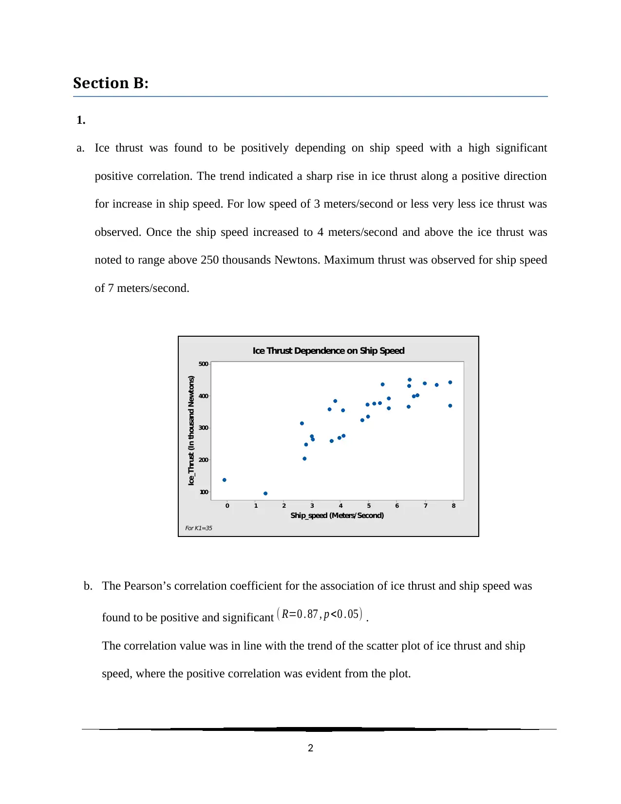
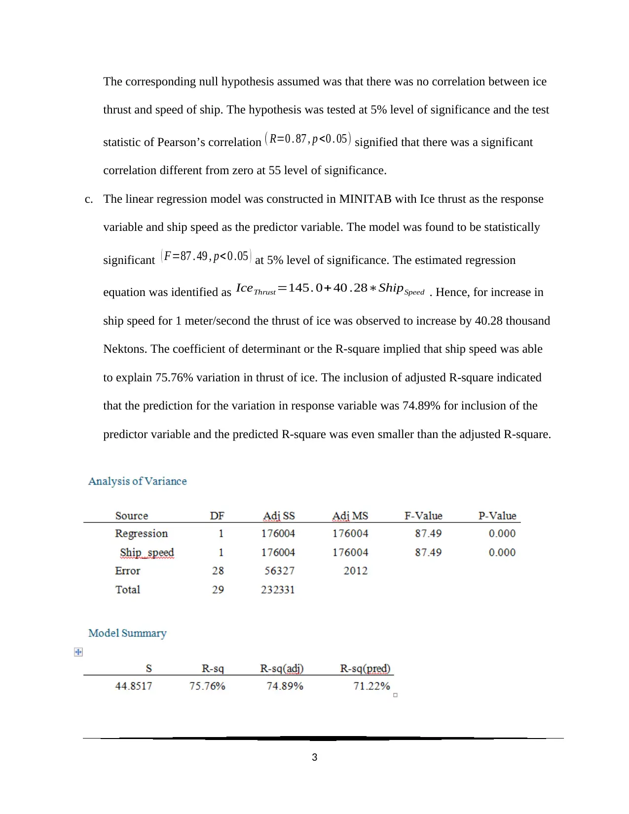
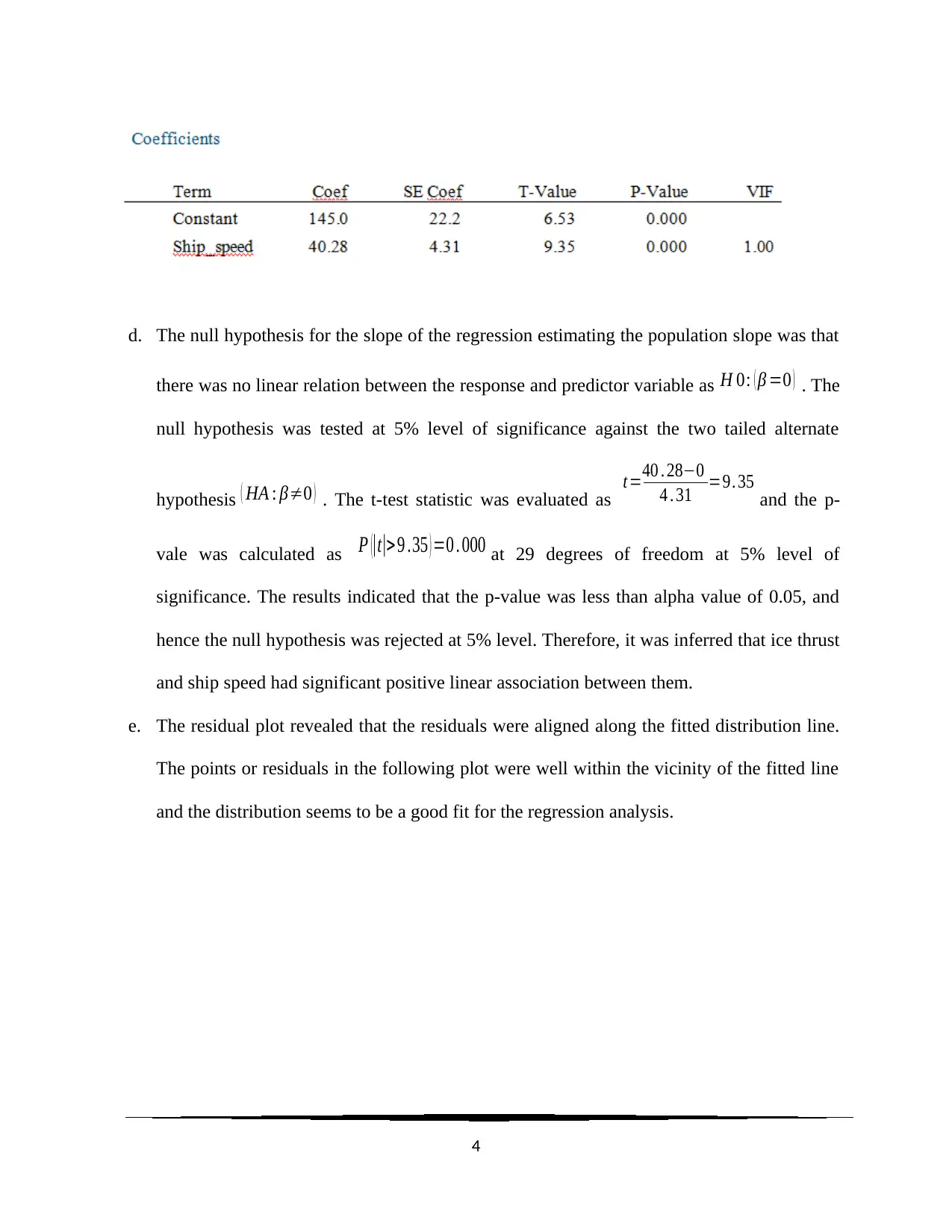
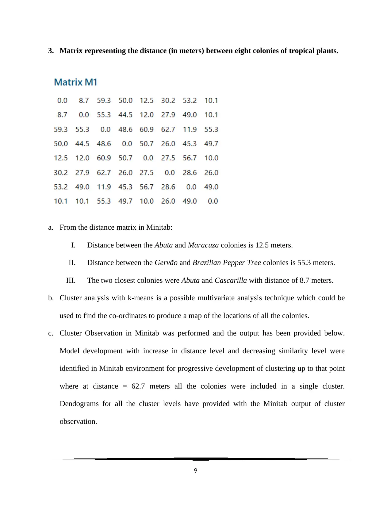
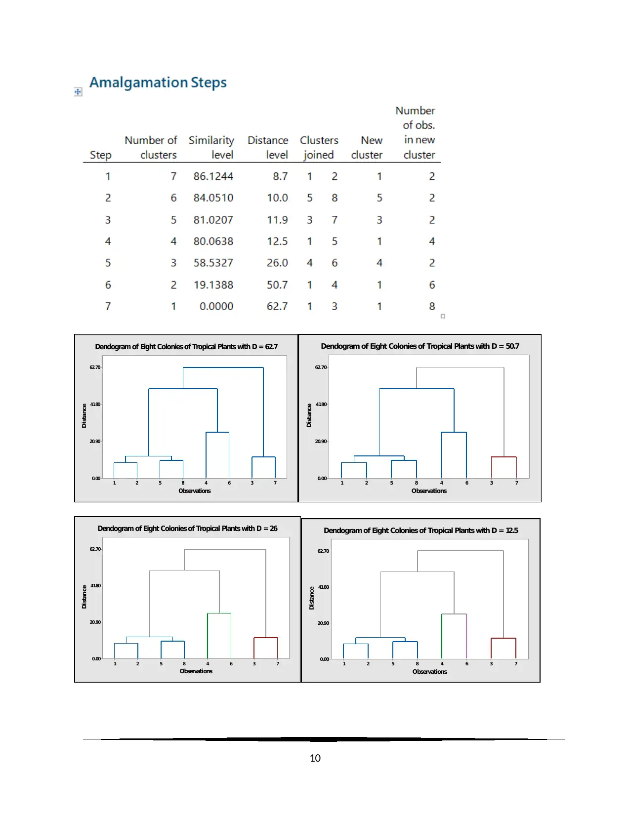
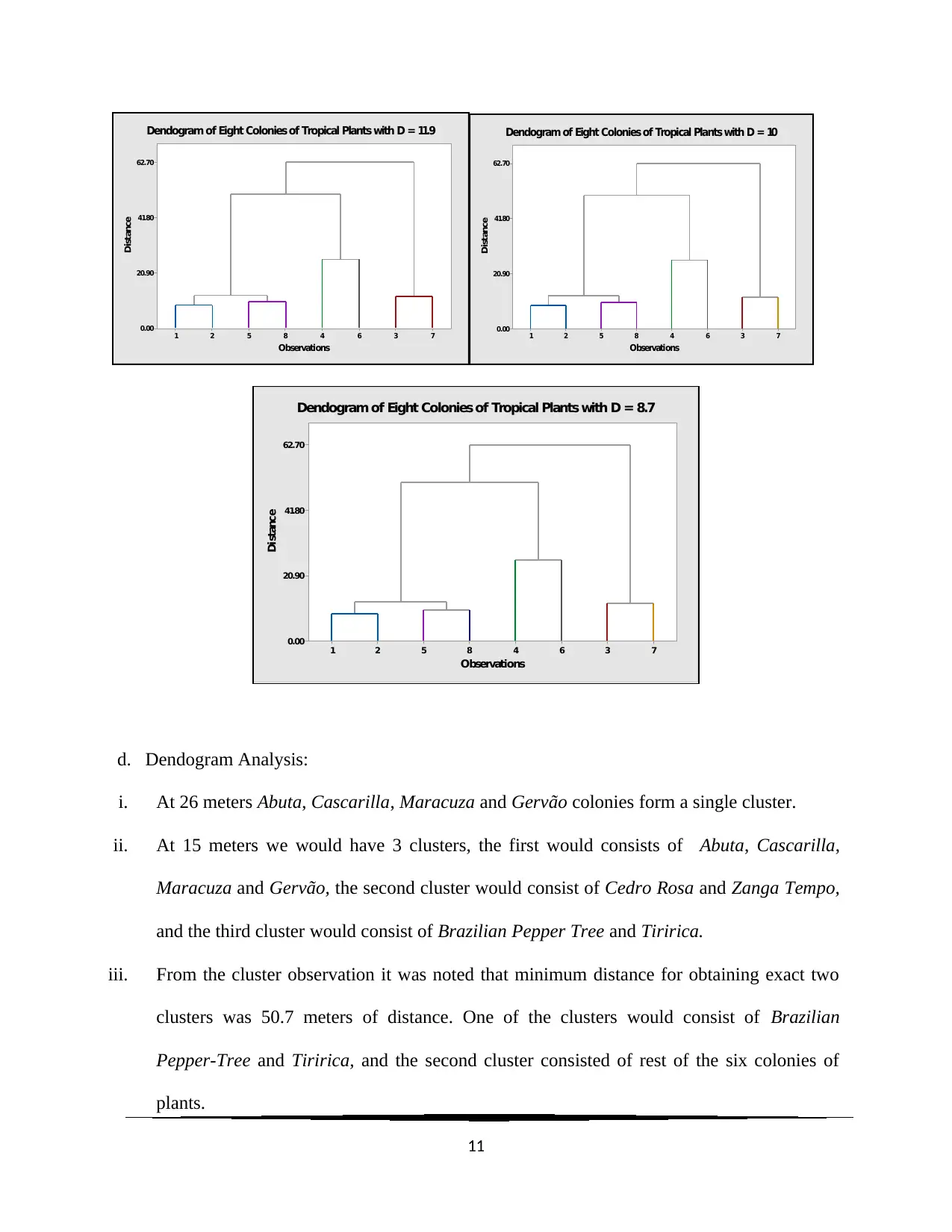
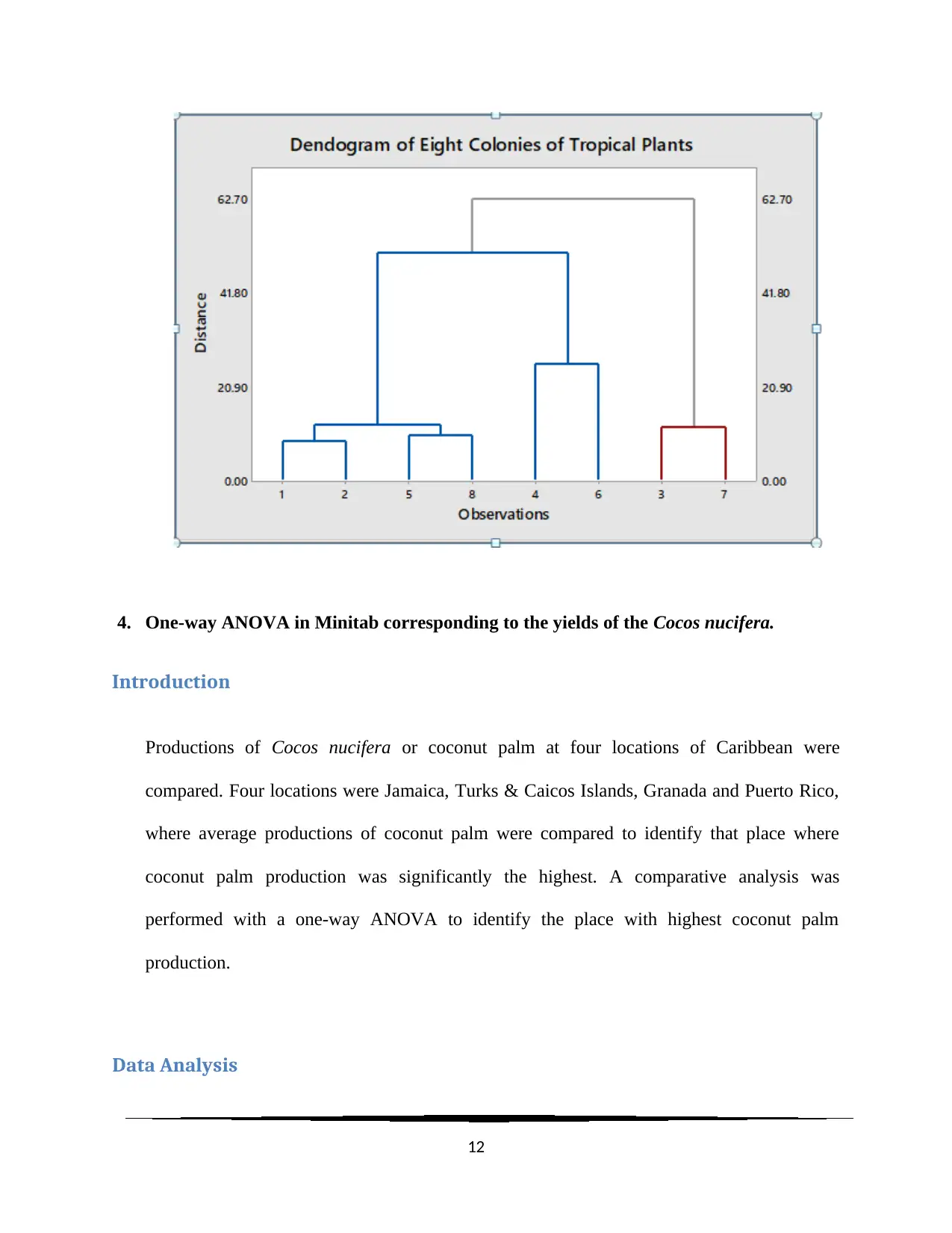
This document presents a comprehensive statistical analysis project, likely for a university-level research methods course. The project explores various statistical techniques including correlation analysis, linear regression modeling, and ANOVA. The analysis begins with examining the relationship between ice thrust and ship speed, utilizing scatter plots, Pearson's correlation, and regression models to quantify the relationship. The project then delves into descriptive statistics and confidence intervals for muzzle velocities of shells, employing histograms and t-tests to assess the data. Finally, the project includes cluster analysis using k-means to analyze the distance between tropical plant colonies and ANOVA to compare coconut palm yields across different locations, providing insights into the data using Minitab output and dendrograms.

RESEARCH METHODS: CRASH COURSE IN STATISTICS
1

Section B:
1.
a. Ice thrust was found to be positively depending on ship speed with a high significant
positive correlation. The trend indicated a sharp rise in ice thrust along a positive direction
for increase in ship speed. For low speed of 3 meters/second or less very less ice thrust was
observed. Once the ship speed increased to 4 meters/second and above the ice thrust was
noted to range above 250 thousands Newtons. Maximum thrust was observed for ship speed
of 7 meters/second.
876543210
500
400
300
200
100
Ship_speed (Meters/Second)
Ice_Thrust (In thousand Newtons)
Ice Thrust Dependence on Ship Speed
For K1=35
b. The Pearson’s correlation coefficient for the association of ice thrust and ship speed was
found to be positive and significant ( R=0 . 87 , p <0 . 05) .
The correlation value was in line with the trend of the scatter plot of ice thrust and ship
speed, where the positive correlation was evident from the plot.
2

The corresponding null hypothesis assumed was that there was no correlation between ice
thrust and speed of ship. The hypothesis was tested at 5% level of significance and the test
statistic of Pearson’s correlation ( R=0 . 87 , p <0 . 05) signified that there was a significant
correlation different from zero at 55 level of significance.
c. The linear regression model was constructed in MINITAB with Ice thrust as the response
variable and ship speed as the predictor variable. The model was found to be statistically
significant ( F=87 . 49 , p< 0 .05 ) at 5% level of significance. The estimated regression
equation was identified as IceThrust =145. 0+40 .28∗ShipSpeed . Hence, for increase in
ship speed for 1 meter/second the thrust of ice was observed to increase by 40.28 thousand
Nektons. The coefficient of determinant or the R-square implied that ship speed was able
to explain 75.76% variation in thrust of ice. The inclusion of adjusted R-square indicated
that the prediction for the variation in response variable was 74.89% for inclusion of the
predictor variable and the predicted R-square was even smaller than the adjusted R-square.
3

d. The null hypothesis for the slope of the regression estimating the population slope was that
there was no linear relation between the response and predictor variable as H 0: ( β =0 ) . The
null hypothesis was tested at 5% level of significance against the two tailed alternate
hypothesis ( HA : β≠0 ) . The t-test statistic was evaluated as t=40 . 28−0
4 . 31 =9. 35 and the p-
vale was calculated as P (|t|>9 .35 ) =0 . 000 at 29 degrees of freedom at 5% level of
significance. The results indicated that the p-value was less than alpha value of 0.05, and
hence the null hypothesis was rejected at 5% level. Therefore, it was inferred that ice thrust
and ship speed had significant positive linear association between them.
e. The residual plot revealed that the residuals were aligned along the fitted distribution line.
The points or residuals in the following plot were well within the vicinity of the fitted line
and the distribution seems to be a good fit for the regression analysis.
4

100500-50-100
99
95
90
80
70
60
50
40
30
20
10
5
1
Residual
Percent
Normal Probability Plot
(response is Ice_Thrust)
From the “Versus fit plot” between the fitted value and the residuals it was evident that the
pattern of residuals was independent that of the fitted values. The residuals were found to
be scatter randomly along the zero line establishing the fact that the relationship between
the response and the predicting variable was linear and the variances of the error term were
equal. The first two residuals were found to be stand out values from the rest of the values.
This trend was also observed in the scatter plot of ice thrust and ship speed. These two
could have been probable outliers for low speed of ships.
f. The estimated regression equation was IceThrust =145. 0+ 40 .28∗ShipSpeed . Now for
ship speed = 6.8 meters per second, the Ice thrust was found to be
IceThrust =145+40 . 28∗6 . 8=418 . 904 or 418904 Newton.
5

500400300200100
100
50
0
-50
-100
Fitted Value
Residual
Versus Fits
(response is Ice_Thrust)
2. Muzzle velocities of 50 shells tested with a new gunpowder:
a. For detail information for the muzzle velocities of the shells with the new gun powder, the
descriptive statistics were scrutinized. The average muzzle velocity was evaluated as 3007.9
meters per second with a standard deviation or root mean square variation in muzzle
velocities of shells as 42 meters per second. The standard deviation suggested that the new
gunpowder had variable effect on the velocities of the shell with majority of the cells
producing a velocity of 3007.9 meters per second on an average. The median velocity of the
distribution was at 3010.5 meters per second with Interquartile velocity spread as 71.3
meters per second. The mean and median values were pretty close to each other, signifying
that the distribution was almost normal with slight positive skewness in the distribution. In
25% cases velocities for shells with new gunpowder was observed to be less than 2972.1
meters per second, whereas, top 25% shells were able to produce a muzzle velocity greater
than 3043.4 meters per second. The fitted curve over the histogram was noted to be in line
6

with the shape of bell curve or normal curve with a single shell producing muzzle velocity
around 3120 meters per second. The 50% of the shells were identified to produce a muzzle
velocity within the range of 2972.1 m/s and 3043.4 m/s.
312030803040300029602920
10
8
6
4
2
0
Mean 3008
StDev 41.98
N 50
Muzzle_Velocities
Frequency
Histogram (with Normal Curve) of Muzzle_Velocities
309030603030300029702940
9
8
7
6
5
4
3
2
1
0
Mean 3006
StDev 38.94
N 49
Muzzle_Velocities
Frequency
Histogram (with Normal Curve) of Muzzle_Velocities
7

b. With 95% confidence it was possible to estimate that the average muzzle velocity of shells
in general would be somewhere between [ x
¿
−t0 . 25∗ s
√ n , x
¿
+t 0 .25∗ s
√ n ] or [ 2996. 0 , 3019 . 9 ]
meters per second. Hence, with 95% confidence it was possible to states that target average
velocity of 3000 m/s was well within the limits of the test data. Therefore, at 5% level of
significance it was not possible to reject the null hypothesis assuming average muzzle
velocity of the shells as 3000 m/s.
c. The null hypothesis was considered as H0: μ=3000 against the two tailed alternate
hypothesis of HA: μ≠3000 at 5% level of significance. The hypothesis was tested by one
sample t-test and the t-statistic was evaluated as ( t=1. 33 , p=0 . 188 ) . There was no statistical
evidence at 5% level of significance that the average muzzle velocity of the shells with a
new variant of gunpowder was different from 3000 meters per second.
The muzzle velocities of the shells were found to be normally distributed and the histogram
plot in part a signified this fact. The velocities were continuous and normally distributed in
nature, establishing the validity of the assumptions of one sample t-test.
8

3. Matrix representing the distance (in meters) between eight colonies of tropical plants.
a. From the distance matrix in Minitab:
I. Distance between the Abuta and Maracuza colonies is 12.5 meters.
II. Distance between the Gervão and Brazilian Pepper Tree colonies is 55.3 meters.
III. The two closest colonies were Abuta and Cascarilla with distance of 8.7 meters.
b. Cluster analysis with k-means is a possible multivariate analysis technique which could be
used to find the co-ordinates to produce a map of the locations of all the colonies.
c. Cluster Observation in Minitab was performed and the output has been provided below.
Model development with increase in distance level and decreasing similarity level were
identified in Minitab environment for progressive development of clustering up to that point
where at distance = 62.7 meters all the colonies were included in a single cluster.
Dendograms for all the cluster levels have provided with the Minitab output of cluster
observation.
9

73648521
62.70
41.80
20.90
0.00
Observations
Distance
Dendogram of Eight Colonies of Tropical Plants with D = 62.7
73648521
62.70
41.80
20.90
0.00
Observations
Distance
Dendogram of Eight Colonies of Tropical Plants with D = 50.7
73648521
62.70
41.80
20.90
0.00
Observations
Distance
Dendogram of Eight Colonies of Tropical Plants with D = 26
73648521
62.70
41.80
20.90
0.00
Observations
Distance
Dendogram of Eight Colonies of Tropical Plants with D = 12.5
10

73648521
62.70
41.80
20.90
0.00
Observations
Distance
Dendogram of Eight Colonies of Tropical Plants with D = 11.9
73648521
62.70
41.80
20.90
0.00
Observations
Distance
Dendogram of Eight Colonies of Tropical Plants with D = 10
73648521
62.70
41.80
20.90
0.00
Observations
Distance
Dendogram of Eight Colonies of Tropical Plants with D = 8.7
d. Dendogram Analysis:
i. At 26 meters Abuta, Cascarilla, Maracuza and Gervão colonies form a single cluster.
ii. At 15 meters we would have 3 clusters, the first would consists of Abuta, Cascarilla,
Maracuza and Gervão, the second cluster would consist of Cedro Rosa and Zanga Tempo,
and the third cluster would consist of Brazilian Pepper Tree and Tiririca.
iii. From the cluster observation it was noted that minimum distance for obtaining exact two
clusters was 50.7 meters of distance. One of the clusters would consist of Brazilian
Pepper-Tree and Tiririca, and the second cluster consisted of rest of the six colonies of
plants.
11

4. One-way ANOVA in Minitab corresponding to the yields of the Cocos nucifera.
Introduction
Productions of Cocos nucifera or coconut palm at four locations of Caribbean were
compared. Four locations were Jamaica, Turks & Caicos Islands, Granada and Puerto Rico,
where average productions of coconut palm were compared to identify that place where
coconut palm production was significantly the highest. A comparative analysis was
performed with a one-way ANOVA to identify the place with highest coconut palm
production.
Data Analysis
12