Decision Analysis for Restaurant Operation and Digital Company - 2018

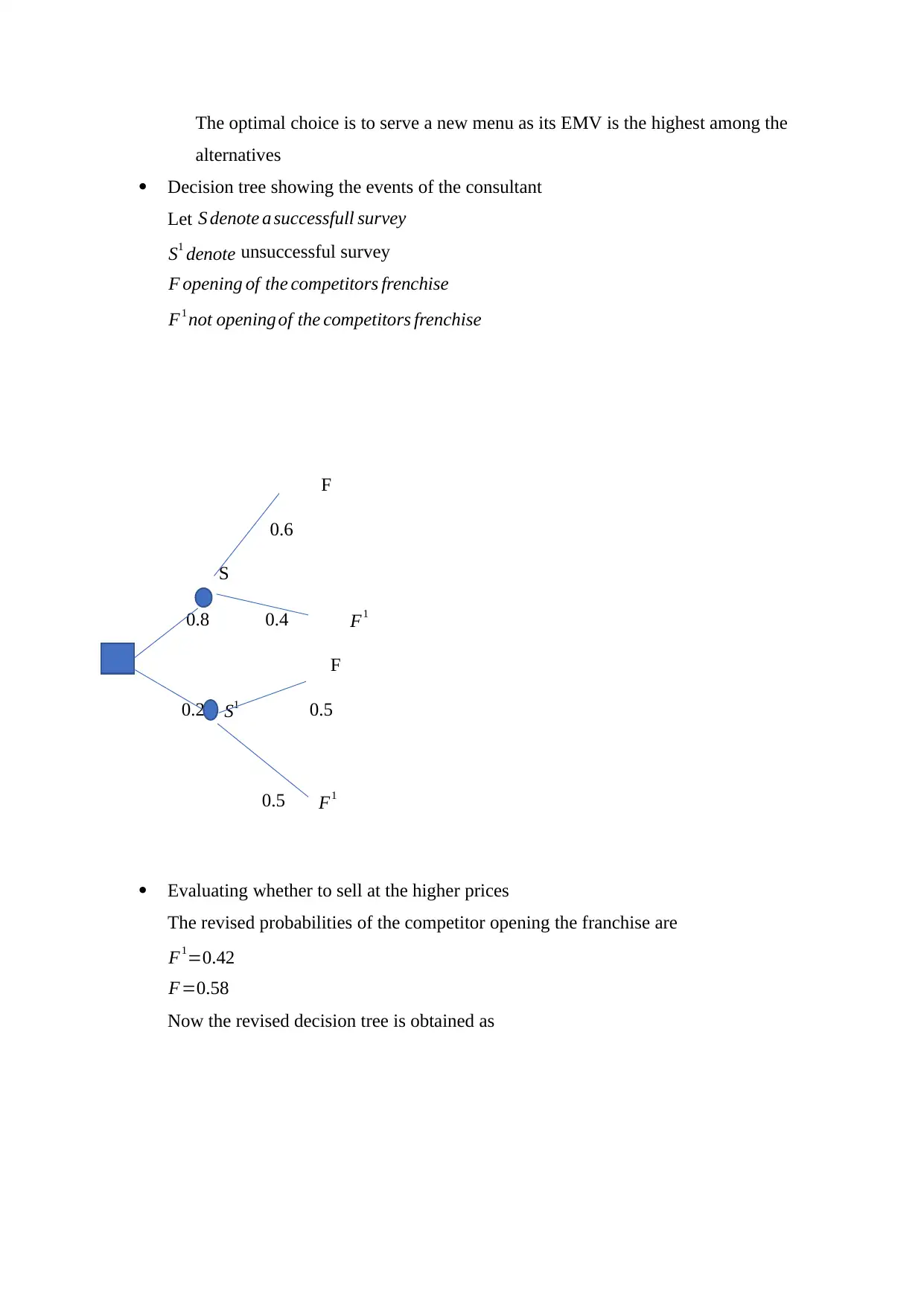
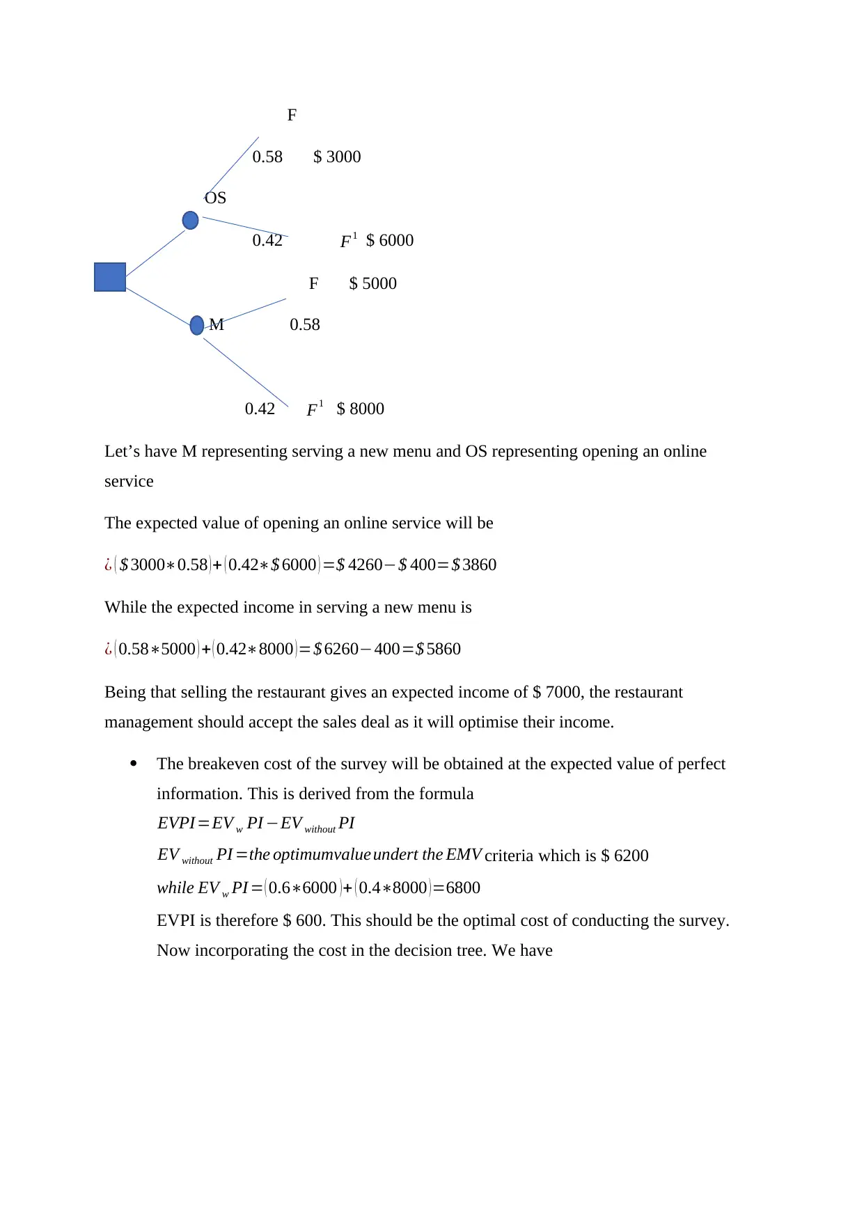
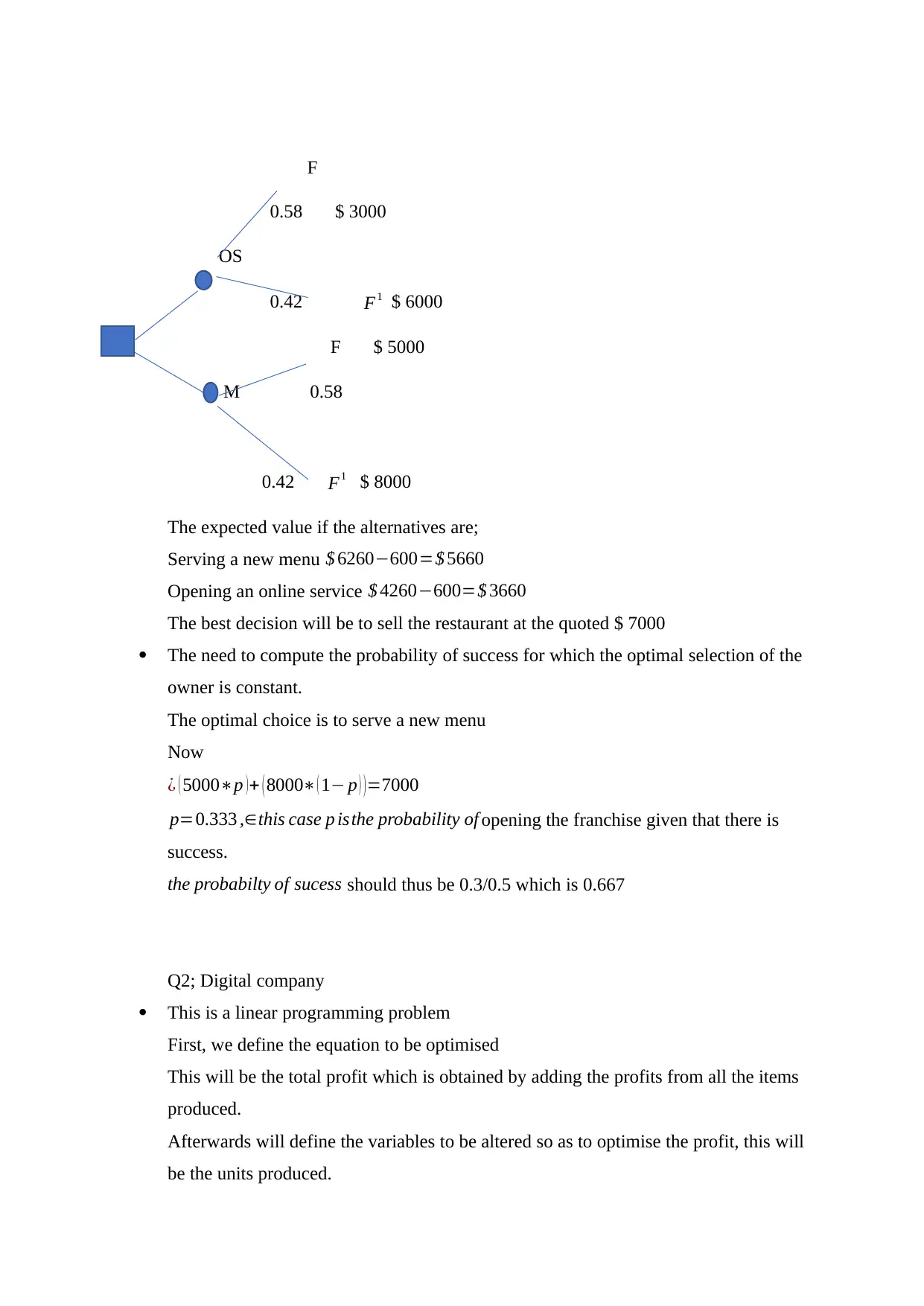
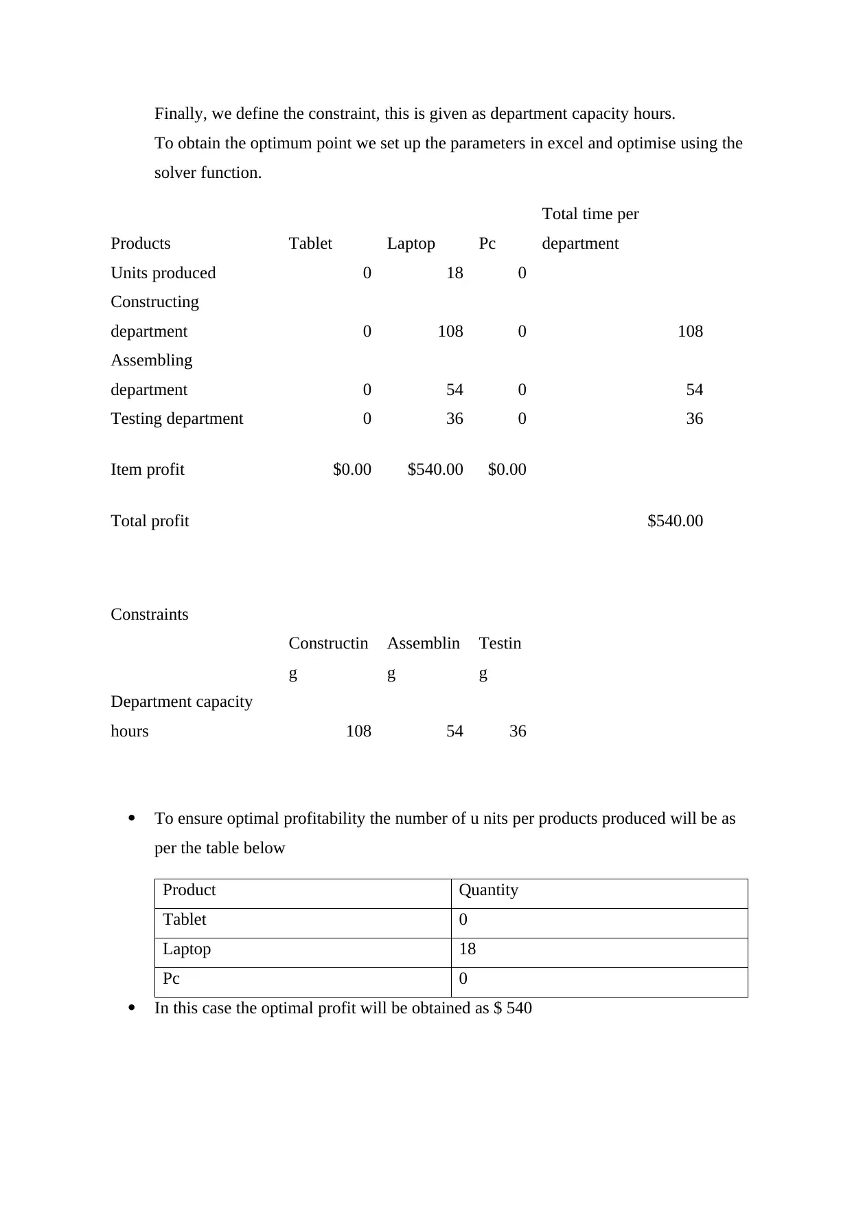
This assignment provides a detailed analysis of decision-making processes for a restaurant operation and a digital company. For the restaurant, it explores various decision models under uncertainty and risk, including maximin, maximax, minimax regret, expected opportunity loss (EOL), and expecte...Read More

Abu Dhabi School of management
Decision Analysis
Group work Sept 2018

Q 1: Restaurant operation decision
 The payoff table
Alternatives Courses of nature
Franchise
opened
Franchise not
opened
Open an online
service
$3000 $6000
Serve a new
menu
$5000 $8000
Sell the
restaurant
$6000 $6000
Prob 0.6 0.4
Optimal decision under the various decision models
Decision making under uncertainty
1. Maximin approach
In this case the decision maker selects the maximum among the worst-case
outcomes
Alternatives Courses of nature
Franchise
opened
Franchise not
opened
Min
Open an online
service
$3000 $6000 $ 3000
Serve a new
menu
$5000 $8000 $5000
Sell the
restaurant
$6000 $6000 $ 6000
Prob 0.6 0.4
The optimal choice under this criterion is to sell the restaurant for $ 6000.

2. Maximax approach
Here the focus us on the best case possible. The maximum among the best options
is thereafter selected.
Alternatives Courses of nature
Franchise
opened
Franchise not
opened
Max
Open an online
service
$3000 $6000 $ 6000
Serve a new
menu
$5000 $8000 $ 8000
Sell the
restaurant
$6000 $6000 $ 6000
Prob 0.6 0.4
The optimal choice is therefore to improve the performance of the restaurant by
serving a new menu. This yield a profit of $ 8000 which is higher than any other
option.
3. Minimax regret approach
In this approach we first compute the regret table as indicated below
Alternatives Courses of nature
Franchise
opened
Franchise not
opened
Max
Open an online
service
$3000 $2000 $ 3000
Serve a new
menu
$1000 0 $ 1000
Sell the
restaurant
0 $2000 $ 2000
Prob 0.6 0.4
The decision selects the alternative with the minimum regret among all the
maximum regrets alternatives.

The optimal course of action is therefore to serve a new menu.
Decision making under risk
4. Expected opportunity loss (EOL)criteria.
We first compute the regret table
Alternatives Courses of nature
Franchise
opened
Franchise not
opened
EOL
Open an online
service
$3000 $2000 $ 2600
Serve a new
menu
$1000 0 $ 600
Sell the
restaurant
0 $2000 $ 800
Prob 0.6 0.4 Prob
Afterwards we calculate the EOL, we thereafter select the option with the
minimum EOL.
The optimal decision is therefore to serve a new menu.
5. Expected monetary value (EMV)
The decision maker computed the expected oncome from each alternative and
select the option which maximises the EMV
Alternatives Courses of nature
Franchise
opened
Franchise not
opened
EMV
Open an online
service
$3000 $6000 $ 4200
Serve a new
menu
$5000 $8000 $ 6200
Sell the
restaurant
$6000 $6000 $ 6000
Prob 0.6 0.4

The optimal choice is to serve a new menu as its EMV is the highest among the
alternatives
 Decision tree showing the events of the consultant
Let S denote a successfull survey
S1 denote unsuccessful survey
F opening of the competitors frenchise
F1 not opening of the competitors frenchise
F
0.6
S
0.8 0.4 F1
F
0.2 S1 0.5
0.5 F1
 Evaluating whether to sell at the higher prices
The revised probabilities of the competitor opening the franchise are
F1=0.42
F=0.58
Now the revised decision tree is obtained as

F
0.58 $ 3000
OS
0.42 F1 $ 6000
F $ 5000
M 0.58
0.42 F1 $ 8000
Let’s have M representing serving a new menu and OS representing opening an online
service
The expected value of opening an online service will be
¿ ( $ 3000∗0.58 ) + ( 0.42∗$ 6000 ) =$ 4260−$ 400=$ 3860
While the expected income in serving a new menu is
¿ ( 0.58∗5000 ) + ( 0.42∗8000 )=$ 6260−400=$ 5860
Being that selling the restaurant gives an expected income of $ 7000, the restaurant
management should accept the sales deal as it will optimise their income.
 The breakeven cost of the survey will be obtained at the expected value of perfect
information. This is derived from the formula
EVPI =EV w PI −EV without PI
EV without PI =the optimumvalueundert the EMV criteria which is $ 6200
while EV w PI = ( 0.6∗6000 )+ ( 0.4∗8000 )=6800
EVPI is therefore $ 600. This should be the optimal cost of conducting the survey.
Now incorporating the cost in the decision tree. We have

F
0.58 $ 3000
OS
0.42 F1 $ 6000
F $ 5000
M 0.58
0.42 F1 $ 8000
The expected value if the alternatives are;
Serving a new menu $ 6260−600=$ 5660
Opening an online service $ 4260−600=$ 3660
The best decision will be to sell the restaurant at the quoted $ 7000
 The need to compute the probability of success for which the optimal selection of the
owner is constant.
The optimal choice is to serve a new menu
Now
¿ ( 5000∗p ) + ( 8000∗ ( 1− p ) )=7000
p=0.333 ,∈this case p isthe probability of opening the franchise given that there is
success.
the probabilty of sucess should thus be 0.3/0.5 which is 0.667
Q2; Digital company
 This is a linear programming problem
First, we define the equation to be optimised
This will be the total profit which is obtained by adding the profits from all the items
produced.
Afterwards will define the variables to be altered so as to optimise the profit, this will
be the units produced.

Finally, we define the constraint, this is given as department capacity hours.
To obtain the optimum point we set up the parameters in excel and optimise using the
solver function.
Products Tablet Laptop Pc
Total time per
department
Units produced 0 18 0
Constructing
department 0 108 0 108
Assembling
department 0 54 0 54
Testing department 0 36 0 36
Item profit $0.00 $540.00 $0.00
Total profit $540.00
Constraints
Constructin
g
Assemblin
g
Testin
g
Department capacity
hours 108 54 36
 To ensure optimal profitability the number of u nits per products produced will be as
per the table below
Product Quantity
Tablet 0
Laptop 18
Pc 0
 In this case the optimal profit will be obtained as $ 540

References
Christian, R. (2007). The Bayesian Choice. New York: Springer.
Martin, P. (2009). An Introduction to Decision Theory. Cambridge University Press.