417 Control Design Project: Robotic Arm Linearization Analysis

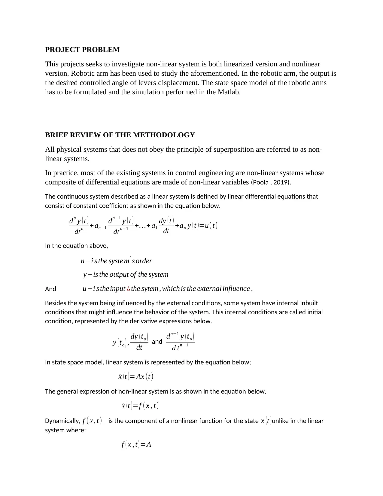
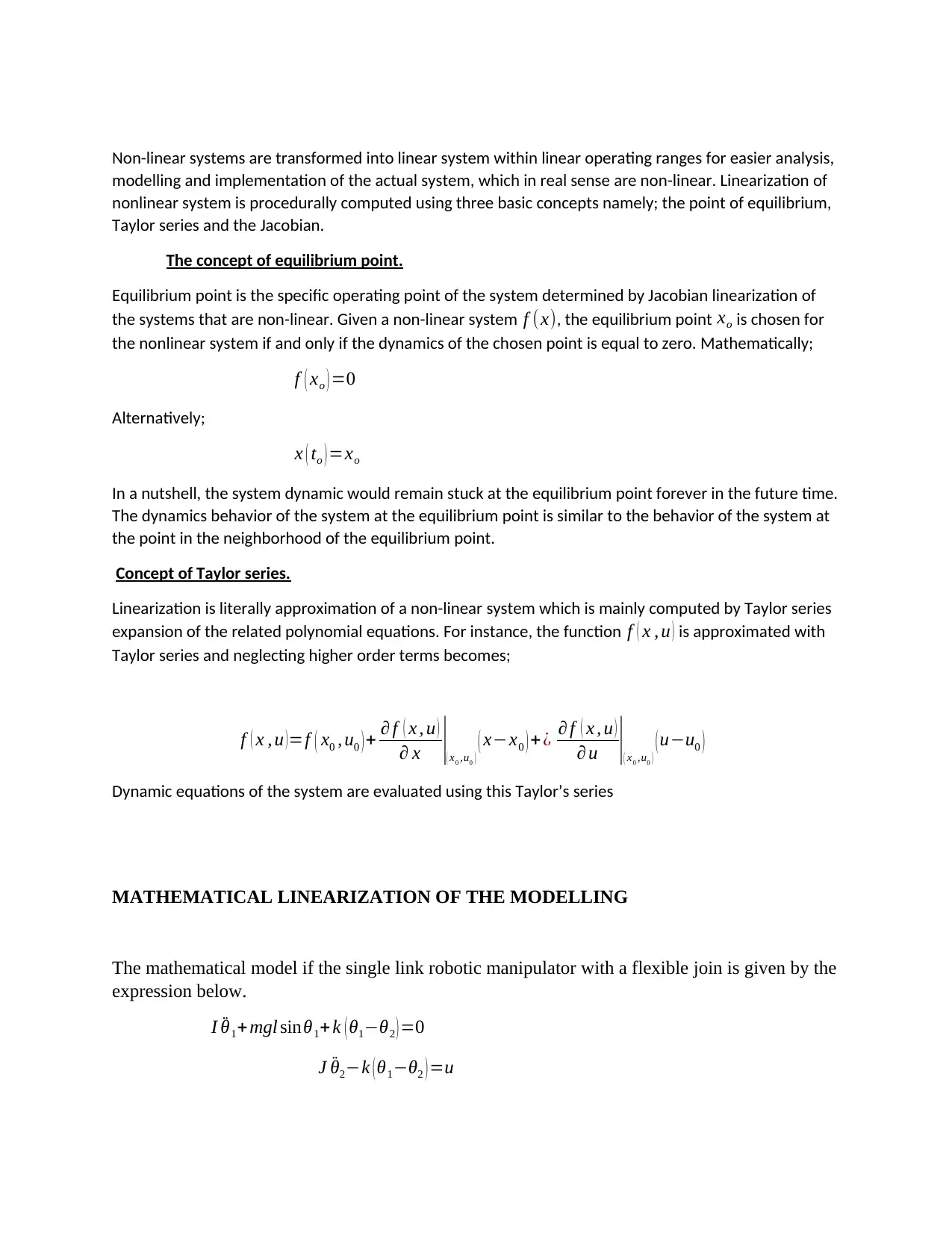
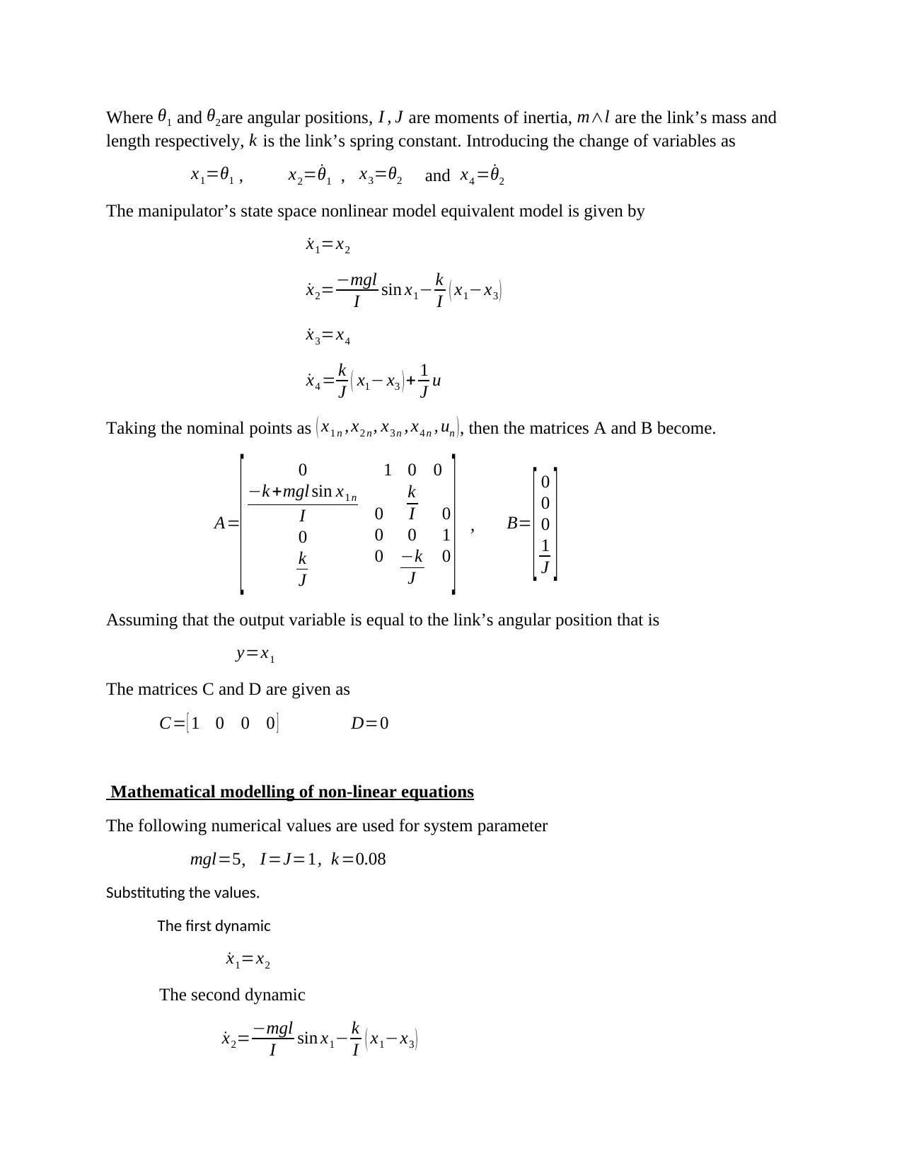
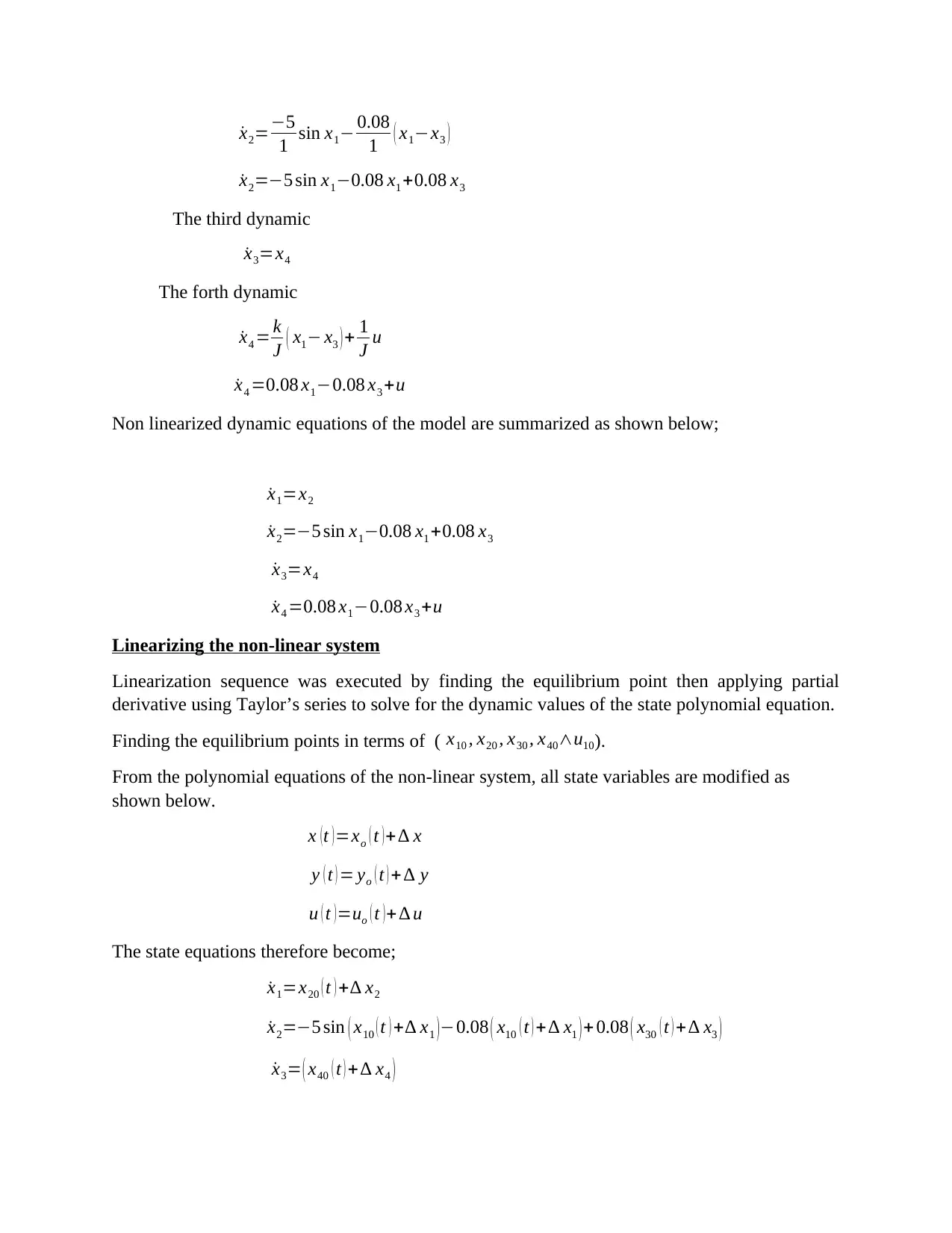
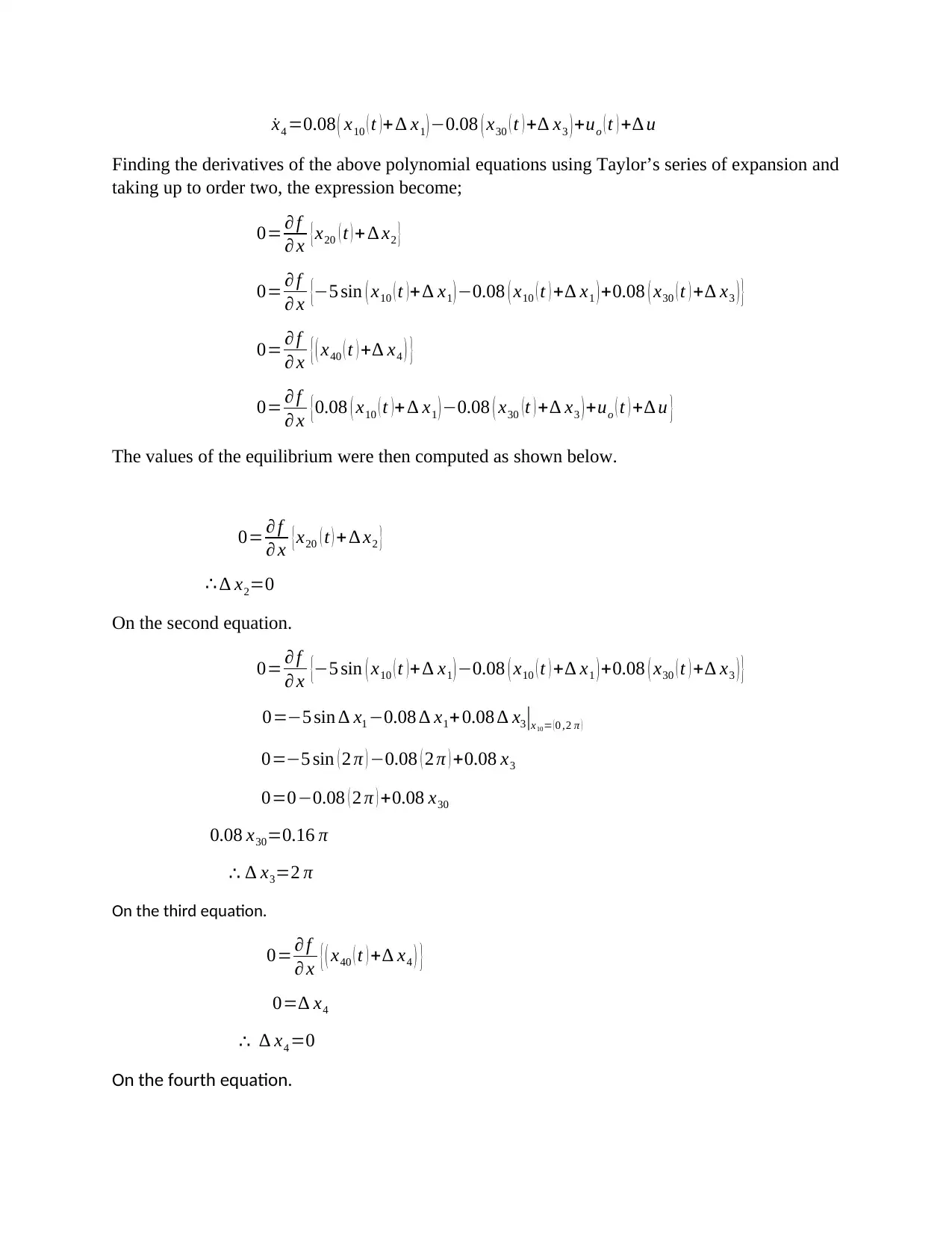
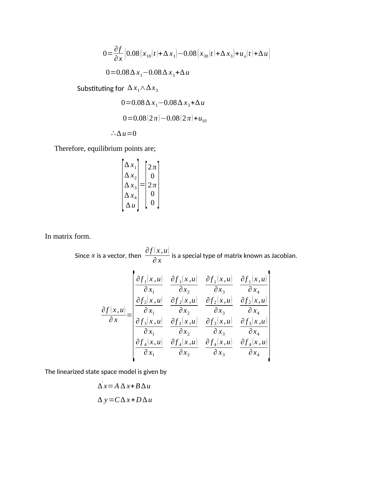
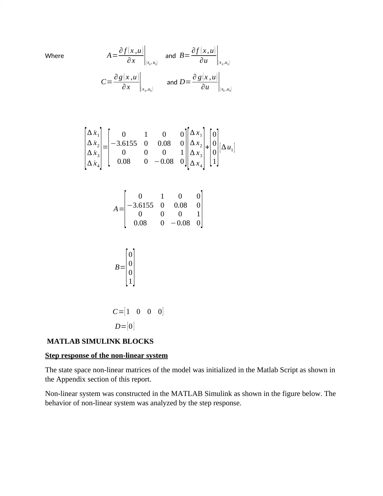
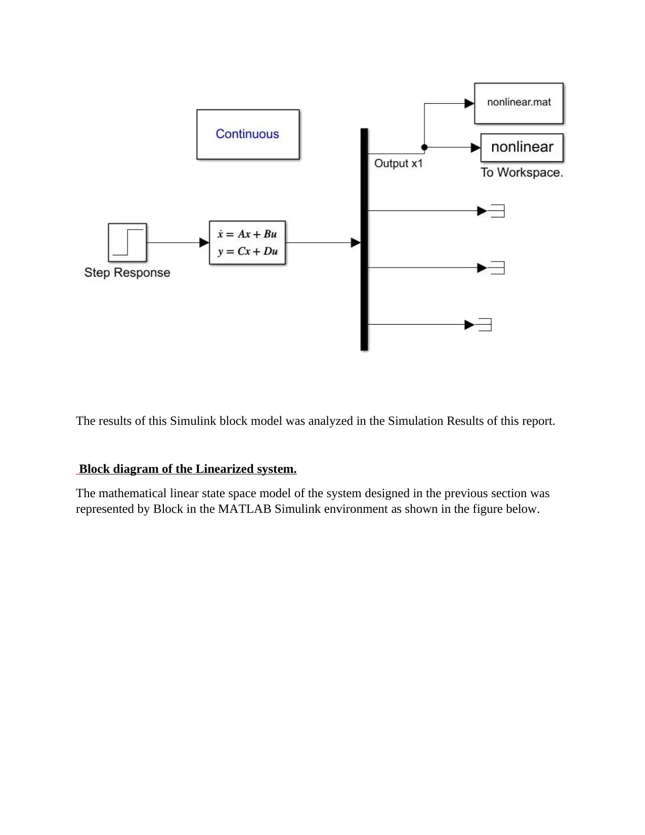
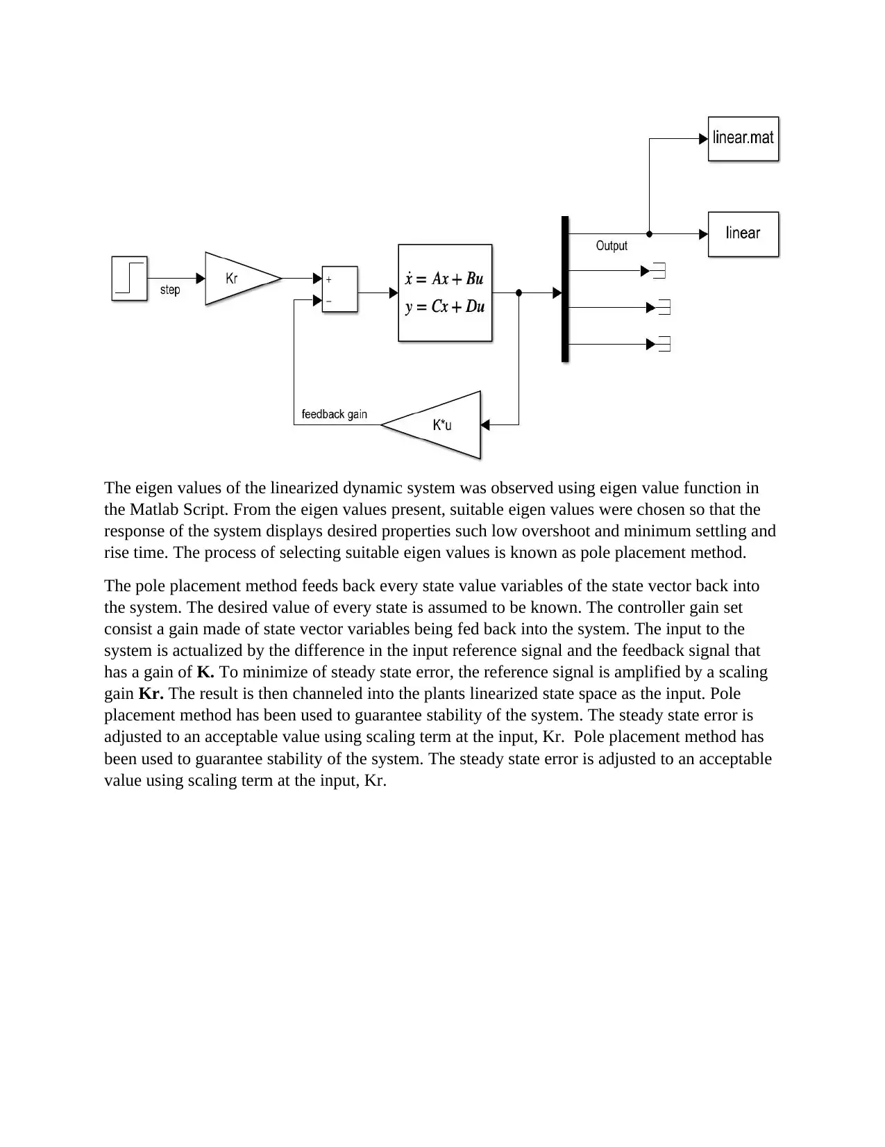
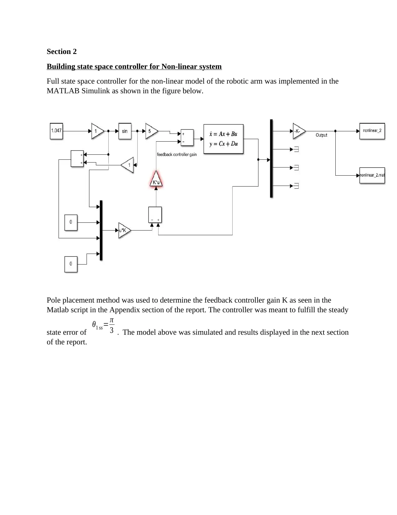
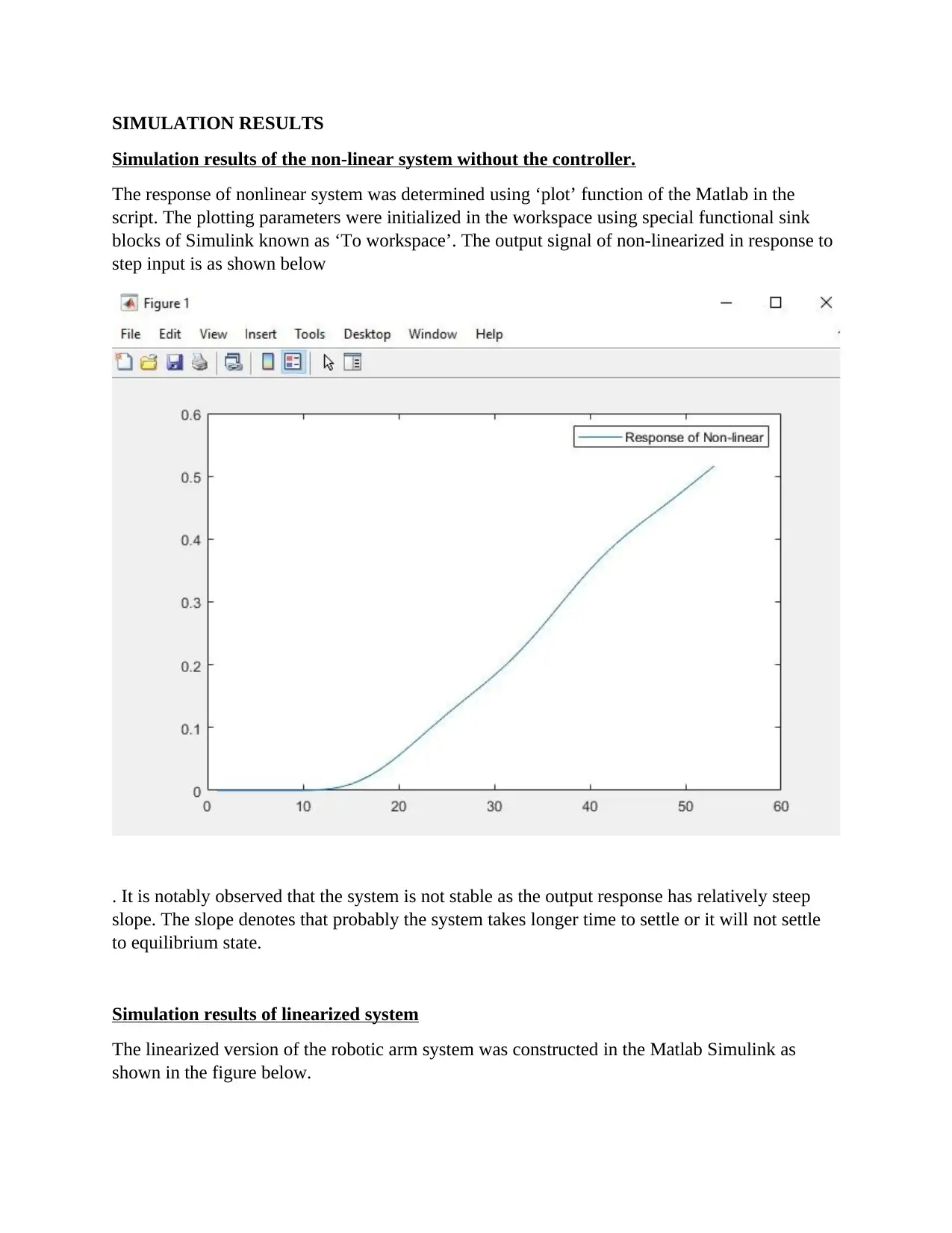
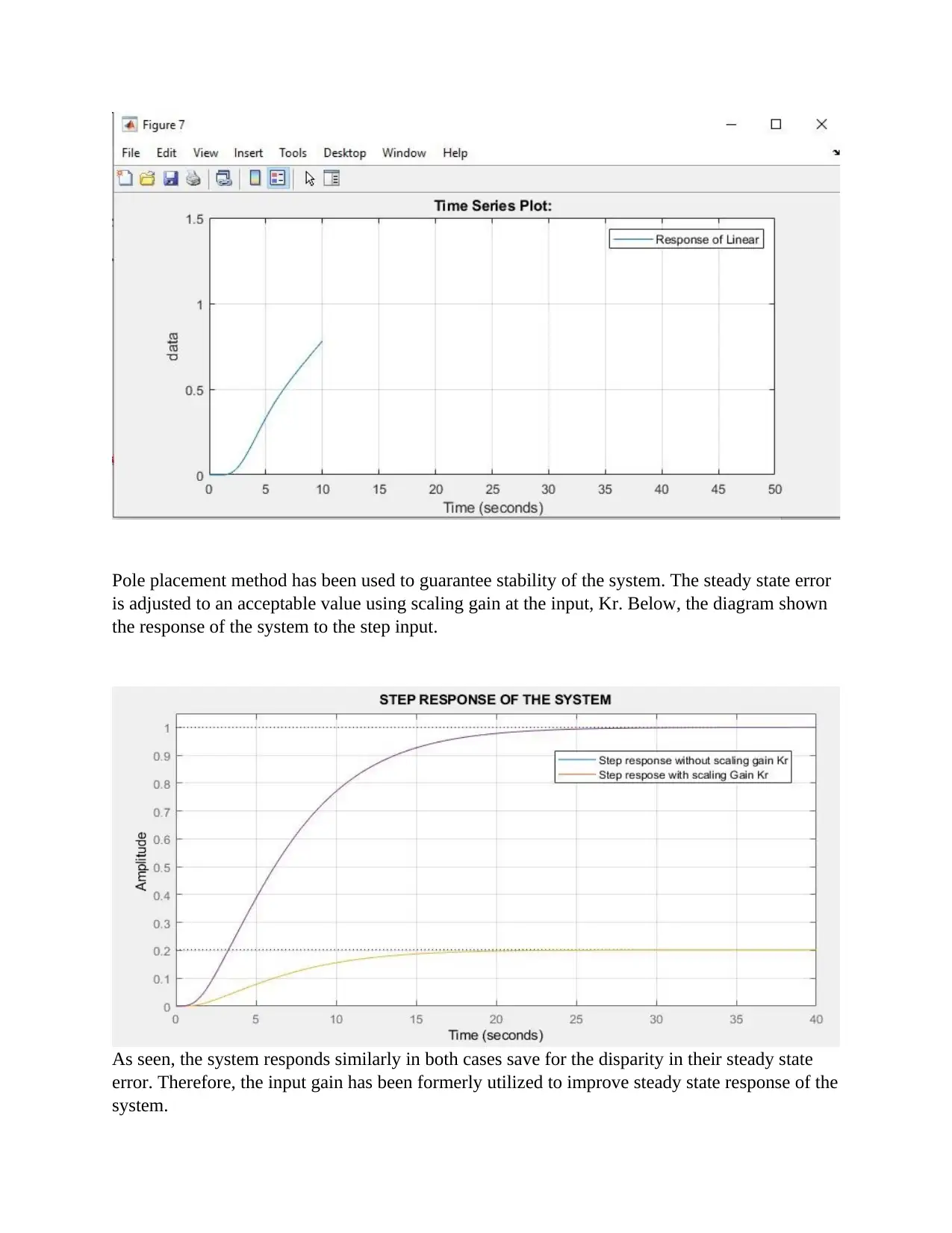
This project investigates the control of a single-link robotic manipulator with a flexible joint. The primary goal is to design a full-state feedback control law for the system by employing linearization around a set point. The project details the mathematical modeling of the robotic arm, including the derivation of state-space models for both the linearized and nonlinear versions of the system. The methodology involves finding equilibrium points, applying Taylor series expansion, and constructing the Jacobian matrix to linearize the nonlinear system. The project utilizes Matlab and Simulink for simulations, including the implementation of a pole placement controller to achieve desired response characteristics such as low overshoot and minimal settling time. The results of the simulations, including step responses for both linearized and controlled systems, are analyzed to evaluate the effectiveness of the control design. The analysis concludes with a comparison of the performance of the linearized and controlled systems, demonstrating the effectiveness of the linearization and control techniques. The project also includes the Matlab scripts used for the simulations.

PROJECT PROBLEM
This projects seeks to investigate non-linear system is both linearized version and nonlinear
version. Robotic arm has been used to study the aforementioned. In the robotic arm, the output is
the desired controlled angle of levers displacement. The state space model of the robotic arms
has to be formulated and the simulation performed in the Matlab.
BRIEF REVIEW OF THE METHODOLOGY
All physical systems that does not obey the principle of superposition are referred to as non-
linear systems.
In practice, most of the existing systems in control engineering are non-linear systems whose
composite of differential equations are made of non-linear variables (Poola , 2019).
The continuous system described as a linear system is defined by linear differential equations that
consist of constant coefficient as shown in the equation below.
dn y ( t )
dtn + an−1
dn−1 y ( t )
dtn−1 +…+ a1
dy ( t )
dt +ao y ( t )=u( t)
In the equation above,
n−i s the syste m' s order
y−is the output of the system
And u−i s the input ¿ the sytem , which is the external influence .
Besides the system being influenced by the external conditions, some system have internal inbuilt
conditions that might influence the behavior of the system. This internal conditions are called initial
condition, represented by the derivative expressions below.
y ( to ) , dy ( to )
dt and dn−1 y ( to )
d tn−1
In state space model, linear system is represented by the equation below;
˙x (t )= Ax (t)
The general expression of non-linear system is as shown in the equation below.
˙x (t )=f (x , t)
Dynamically, f ( x , t ) is the component of a nonlinear function for the state x (t )unlike in the linear
system where;
f ( x , t ) =A

Non-linear systems are transformed into linear system within linear operating ranges for easier analysis,
modelling and implementation of the actual system, which in real sense are non-linear. Linearization of
nonlinear system is procedurally computed using three basic concepts namely; the point of equilibrium,
Taylor series and the Jacobian.
The concept of equilibrium point.
Equilibrium point is the specific operating point of the system determined by Jacobian linearization of
the systems that are non-linear. Given a non-linear system f (x), the equilibrium point xo is chosen for
the nonlinear system if and only if the dynamics of the chosen point is equal to zero. Mathematically;
f ( xo ) =0
Alternatively;
x ( to ) =xo
In a nutshell, the system dynamic would remain stuck at the equilibrium point forever in the future time.
The dynamics behavior of the system at the equilibrium point is similar to the behavior of the system at
the point in the neighborhood of the equilibrium point.
Concept of Taylor series.
Linearization is literally approximation of a non-linear system which is mainly computed by Taylor series
expansion of the related polynomial equations. For instance, the function f ( x , u ) is approximated with
Taylor series and neglecting higher order terms becomes;
f ( x , u )=f ( x0 , u0 ) + ∂ f ( x , u )
∂ x |( x0 ,u0 )
( x−x0 ) +¿ ∂ f ( x , u )
∂ u |( x0 ,u0 )
( u−u0 )
Dynamic equations of the system are evaluated using this Taylor’s series
MATHEMATICAL LINEARIZATION OF THE MODELLING
The mathematical model if the single link robotic manipulator with a flexible join is given by the
expression below.
I ¨θ1+mgl sinθ1+ k ( θ1−θ2 ) =0
J ¨θ2−k ( θ1−θ2 ) =u

Where θ1 and θ2are angular positions, I , J are moments of inertia, m∧l are the link’s mass and
length respectively, k is the link’s spring constant. Introducing the change of variables as
x1=θ1 , x2= ˙θ1 , x3=θ2 and x4 = ˙θ2
The manipulator’s state space nonlinear model equivalent model is given by
˙x1=x2
˙x2=−mgl
I sin x1− k
I ( x1−x3 )
˙x3=x4
˙x4 = k
J ( x1− x3 ) + 1
J u
Taking the nominal points as ( x1 n , x2 n , x3 n , x4 n , un ), then the matrices A and B become.
A=
[ 0 1 0 0
−k +mgl sin x1 n
I
0
k
J
0
0
0
k
I
0
−k
J
0
1
0 ] , B=
[ 0
0
0
1
J ]
Assuming that the output variable is equal to the link’s angular position that is
y=x1
The matrices C and D are given as
C= [ 1 0 0 0 ] D=0
Mathematical modelling of non-linear equations
The following numerical values are used for system parameter
mgl=5, I =J=1, k =0.08
Substituting the values.
The first dynamic
˙x1=x2
The second dynamic
˙x2=−mgl
I sin x1− k
I ( x1−x3 )

˙x2=−5
1 sin x1− 0.08
1 ( x1−x3 )
˙x2=−5 sin x1−0.08 x1 +0.08 x3
The third dynamic
˙x3=x4
The forth dynamic
˙x4 = k
J ( x1− x3 ) + 1
J u
˙x4 =0.08 x1−0.08 x3 +u
Non linearized dynamic equations of the model are summarized as shown below;
˙x1=x2
˙x2=−5 sin x1−0.08 x1 +0.08 x3
˙x3=x4
˙x4 =0.08 x1−0.08 x3 +u
Linearizing the non-linear system
Linearization sequence was executed by finding the equilibrium point then applying partial
derivative using Taylor’s series to solve for the dynamic values of the state polynomial equation.
Finding the equilibrium points in terms of ( x10 , x20 , x30 , x40∧u10).
From the polynomial equations of the non-linear system, all state variables are modified as
shown below.
x (t )=xo ( t )+ ∆ x
y ( t ) = yo ( t ) + ∆ y
u ( t ) =uo ( t ) + ∆ u
The state equations therefore become;
˙x1=x20 ( t ) +∆ x2
˙x2=−5 sin ( x10 ( t ) +∆ x1 )−0.08 ( x10 ( t ) +∆ x1 )+ 0.08 ( x30 ( t ) +∆ x3 )
˙x3= ( x40 ( t ) +∆ x4 )

˙x4 =0.08 ( x10 ( t )+ ∆ x1 )−0.08 ( x30 ( t ) +∆ x3 )+uo ( t ) +∆ u
Finding the derivatives of the above polynomial equations using Taylor’s series of expansion and
taking up to order two, the expression become;
0= ∂ f
∂ x {x20 ( t ) + ∆ x2 }
0= ∂ f
∂ x {−5 sin ( x10 ( t )+∆ x1 )−0.08 ( x10 ( t ) +∆ x1 )+0.08 ( x30 ( t ) +∆ x3 ) }
0= ∂ f
∂ x { ( x40 ( t ) +∆ x4 ) }
0= ∂ f
∂ x {0.08 ( x10 ( t )+ ∆ x1 )−0.08 ( x30 (t ) +∆ x3 )+uo ( t ) +∆ u }
The values of the equilibrium were then computed as shown below.
0= ∂ f
∂ x {x20 ( t ) + ∆ x2 }
∴ ∆ x2=0
On the second equation.
0= ∂ f
∂ x {−5 sin ( x10 ( t )+∆ x1 )−0.08 ( x10 ( t ) +∆ x1 )+0.08 ( x30 ( t ) +∆ x3 ) }
0=−5 sin ∆ x1 −0.08 ∆ x1+ 0.08 ∆ x3|x10= (0 ,2 π )
0=−5 sin ( 2 π ) −0.08 ( 2 π ) +0.08 x3
0=0−0.08 ( 2 π ) +0.08 x30
0.08 x30=0.16 π
∴ ∆ x3=2 π
On the third equation.
0= ∂ f
∂ x { ( x40 ( t ) +∆ x4 ) }
0=∆ x4
∴ ∆ x4 =0
On the fourth equation.

0= ∂ f
∂ x {0.08 ( x10 ( t )+ ∆ x1 )−0.08 ( x30 (t ) +∆ x3 )+uo ( t ) +∆ u }
0=0.08 ∆ x1−0.08 ∆ x3 +∆ u
Substituting for ∆ x1∧∆ x3
0=0.08 ∆ x1−0.08 ∆ x3 +∆ u
0=0.08 ( 2 π ) −0.08 ( 2 π ) +u10
∴ ∆ u=0
Therefore, equilibrium points are;
[∆ x1
∆ x2
∆ x3
∆ x4
∆ u ]=
[2 π
0
2 π
0
0 ]
In matrix form.
Since x is a vector, then ∂ f ( x , u )
∂ x is a special type of matrix known as Jacobian.
∂ f ( x , u )
∂ x =
[ ∂ f 1 ( x , u )
∂ x1
∂ f 1 ( x ,u )
∂ x2
∂ f 1 ( x , u )
∂ x3
∂ f 1 ( x , u )
∂ x4
∂ f 2 ( x , u )
∂ x1
∂ f 2 ( x ,u )
∂ x2
∂ f 2 ( x , u )
∂ x3
∂ f 2 ( x , u )
∂ x4
∂ f 3 ( x , u )
∂ x1
∂ f 4 ( x , u )
∂ x1
∂ f 3 ( x ,u )
∂ x2
∂ f 4 ( x ,u )
∂ x2
∂ f 3 ( x , u )
∂ x3
∂ f 4 ( x , u )
∂ x3
∂ f 3 ( x ,u )
∂ x4
∂ f 4 ( x , u )
∂ x4
]The linearized state space model is given by
˙∆ x= A ∆ x+B ∆ u
∆ y =C ∆ x + D ∆ u

Where A= ∂ f ( x ,u )
∂ x |( x0 , u0 )
and B= ∂ f ( x , u )
∂u |( x0 ,u0 )
C= ∂ g ( x ,u )
∂ x |( x0 ,u0 )
and D= ∂ g ( x , u )
∂u |( x0 ,u0 )
[∆ ˙x1
∆ ˙x2
∆ ˙x3
∆ ˙x4
]=
[ 0
−3.6155
0
0.08
1
0
0
0
0
0.08
0
−0.08
0
0
1
0 ] [∆ x1
∆ x2
∆ x3
∆ x4
]+
[0
0
0
1 ] [ ∆ u1 ]
A=
[ 0
−3.6155
0
0.08
1
0
0
0
0
0.08
0
−0.08
0
0
1
0 ]
B=
[0
0
0
1 ]
C= [ 1 0 0 0 ]
D= [ 0 ]
MATLAB SIMULINK BLOCKS
Step response of the non-linear system
The state space non-linear matrices of the model was initialized in the Matlab Script as shown in
the Appendix section of this report.
Non-linear system was constructed in the MATLAB Simulink as shown in the figure below. The
behavior of non-linear system was analyzed by the step response.

The results of this Simulink block model was analyzed in the Simulation Results of this report.
Block diagram of the Linearized system.
The mathematical linear state space model of the system designed in the previous section was
represented by Block in the MATLAB Simulink environment as shown in the figure below.

The eigen values of the linearized dynamic system was observed using eigen value function in
the Matlab Script. From the eigen values present, suitable eigen values were chosen so that the
response of the system displays desired properties such low overshoot and minimum settling and
rise time. The process of selecting suitable eigen values is known as pole placement method.
The pole placement method feeds back every state value variables of the state vector back into
the system. The desired value of every state is assumed to be known. The controller gain set
consist a gain made of state vector variables being fed back into the system. The input to the
system is actualized by the difference in the input reference signal and the feedback signal that
has a gain of K. To minimize of steady state error, the reference signal is amplified by a scaling
gain Kr. The result is then channeled into the plants linearized state space as the input. Pole
placement method has been used to guarantee stability of the system. The steady state error is
adjusted to an acceptable value using scaling term at the input, Kr. Pole placement method has
been used to guarantee stability of the system. The steady state error is adjusted to an acceptable
value using scaling term at the input, Kr.

Section 2
Building state space controller for Non-linear system
Full state space controller for the non-linear model of the robotic arm was implemented in the
MATLAB Simulink as shown in the figure below.
Pole placement method was used to determine the feedback controller gain K as seen in the
Matlab script in the Appendix section of the report. The controller was meant to fulfill the steady
state error of θ1 ss= π
3 . The model above was simulated and results displayed in the next section
of the report.

SIMULATION RESULTS
Simulation results of the non-linear system without the controller.
The response of nonlinear system was determined using ‘plot’ function of the Matlab in the
script. The plotting parameters were initialized in the workspace using special functional sink
blocks of Simulink known as ‘To workspace’. The output signal of non-linearized in response to
step input is as shown below
. It is notably observed that the system is not stable as the output response has relatively steep
slope. The slope denotes that probably the system takes longer time to settle or it will not settle
to equilibrium state.
Simulation results of linearized system
The linearized version of the robotic arm system was constructed in the Matlab Simulink as
shown in the figure below.

Pole placement method has been used to guarantee stability of the system. The steady state error
is adjusted to an acceptable value using scaling gain at the input, Kr. Below, the diagram shown
the response of the system to the step input.
As seen, the system responds similarly in both cases save for the disparity in their steady state
error. Therefore, the input gain has been formerly utilized to improve steady state response of the
system.

The desired response characteristics were achieved as shown in the figure below.
The system has zero overshoot, 11.4 seconds rise time and zero steady state error. Therefore, the
system is stable, the fact which is observable from the system response.
Simulation results of controlled non-linear system
The system was modelled with dynamic variable of the state vectors. By incorporating the
controller, non-linear controlled robotic arm system is as shown in the figure below.
T
he plot function was used to ‘plot’ the graph above.

For analysis purpose, the same graph was redrawn using ‘step’ function and the resultant is as
shown in the graph below.
The system is stable as it has zero steady space error. However, there is an element of 20%
overshoot unlike in the linearized controlled system.
CONCLUSION.
The analysis of the robotic arm was investigated both in non-linearized environment and
linearized equivalent. The linearization was implemented mathematically by use of equilibrium
values of the dynamic variable. Combination of Taylor’s series and Jacobian matrices resulted to
linearized state matrices of the system. The linearized and non-linear system were then
successfully implemented in the Matlab. In th Matlab environment, the system was partially
constructed in the Matlab script and Matlab Simulink. The response of the system was analyzed
using step input as the reference signal.

REFERENCES
Poola and Horowitz. (2019). Jacobian Linearizations, equilibrium points. [online] Available at:
https://www.cds.caltech.edu/~murray/courses/cds101/fa02/caltech/pph02-ch19-23.pdf [Accessed 18
Oct. 2019].
APPENDIX 1
Non-Linear and Linearized system.
clear all
clc
%s=tf('s')
%%%%%%%%%%%%%%%%%%5
%%%Initialization of the system variables
mgl=5;
I=1;
J=1;
%%%%%%%%%%%%%%%%%%%%%%%%%%%%%%%%%%%%%%%%%
%Initialization of the State matrices
%%%%%%%%%%%%%%%%%%%%%%%%%%%%%%%%
A=[0 1 0 0;-3.6155 0 0.08 0;0 0 0 1;0.08 0 -0.08 0]
B=[0;0;0;1]
C=[1 0 0 0]
D=[0]
%%%%%%%%%%%%%%%%%%%%%
% creating state space model
sys=ss(A,B,C,D);
%%%%%%%%%%%%%%%%%%%%%%%%%%%%%%%
%%plotting Simulink results in
%%
out = sim('NON_LINEAR_1');
load('nonlinear.mat')
figure;
plot(out.nonlinear)
axis([0 50 0 1.5])
grid on
legend('Response of Non-linear')
%%
%PLotting step response
figure

step(sys)
axis([0 50 0 1.5])
%%
%%checking open loop eigen valuues
E=eig(A);
%%%
%desired closed loop eigen values
P=[-1+1.90i,-1-1.90i,-0.286,-0.3];
%solve for value of K using pole placement
K=place(A,B,P);
%check for closed loop eigenvalues
A_cl=A-B*K;
E_cl=eig(A_cl);
%creat closed loop system
sys_cl=ss(A_cl,B,C,D)
%Finding the dc gain and inverting to get scaling factor
Kdc=dcgain(sys_cl);
%Finding the scaling inputfactor
Kr=1/Kdc;
%scaled system
sys_scaled=ss(A_cl,B*Kr,C,D)
%%
%Plotting simulink signal
out = sim('LINEAR_1');
load('linear.mat')
figure
plot(out.linear)
axis([0 50 0 1.5])
grid on
legend('Response of Linear')
%%
%Plotting step response of the scaled system
figure
step(sys_scaled)
axis([0 50 0 1.5])
%%
%%END
%%
APPENDIX 2
Controller of Non-linearized system
clear all
clc
%s=tf('s');

mgl=5;
I=1;
J=1;
%%
%%DEFINING THE MATRIX
%%%%%%%%
A1=[0 1 0 0;-2.58 0 0.08 0;0 0 0 1;0.08 0 0.08 0]
B1=[0;0;0;1]
C1=[1 0 0 0]
D1=[0]
%%%%%%%%%%%%%
% CREATING STATE SPACE MODEL
sys1=ss(A1,B1,C1,D1)
%%
%%%CHECKING EIGEN VALUES OF THE OPEN LOOP
E1=eig(A1)
%%%%%%%%%%%%%%%%%%%%%%%%%%%%%%%%%%%%%%%%%%%%%
%DESIRED CLOSED LOOP TRANSFER FUCNTION
P1=[-1+1.60i,-1-1.60i,-2.86,-3];
%%
%DESIGNING THE CONTROLLER K USING POLE PLACEMENT METHOD
K1=place(A1,B1,P1)
%CHECKING CLOSED LOOP EIGEN VALUES FOR STABILITY
A_cl1=A1-B1*K1
E_cl1=eig(A_cl1)
%CREATING STATE SPACE CLOSED LOOP SYSTEM WITH A FEEDBACK COTROLLER
sys_cl1=ss(A_cl1,B1,C1,D1)
%STEP RESPONSE OF THE CLOSED LOOP
figure
step(sys_cl1)
grid on
hold on
%%
%FINIDNG D.C GAIN AND INVERTING TO FORM INPUT GAIN SALING FACTOR FOR BETTER
%RESPONSE
Kdc=dcgain(sys_cl1)
%INPUT SCALING FACTOR.

Kr_1=1/Kdc
%SCALED SYSTEM
sys_scaled1=ss(A_cl1,B1*Kr_1,C1,D1)
%%
% RESPONSE OF THE SCALED CLOSED LOOP SYSTEM IN SIMULINK
out = sim('NON_LINEAR_2');
load('nonlinear_2.mat')
%subplot(2,1,1)
figure;
plot(out.nonlinear_2)
axis([0 50 0 1.5])
grid on
legend('Response of Non-linear_2')
%%
%STEP RESPONSE OF THE SYSTEM
figure
step(sys_scaled1)
axis([0 50 0 1.5])
grid on
legend('Non Linear Controller')
title('STEP RESPONSE OF THE SYSTEM')
%THE END