RStudio: Analysis of Energy Consumption (MMBtu_TOTAL) Data Report

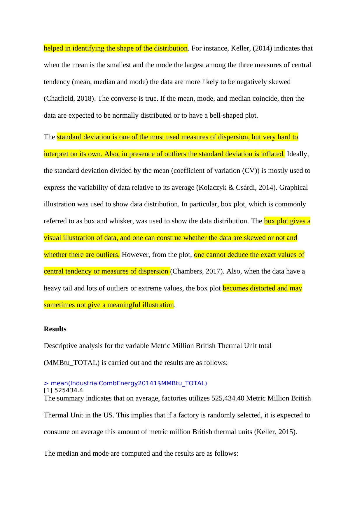
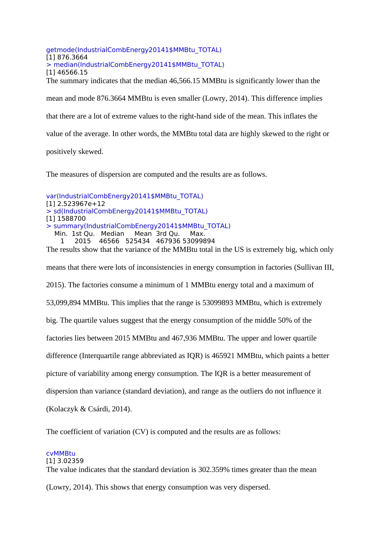
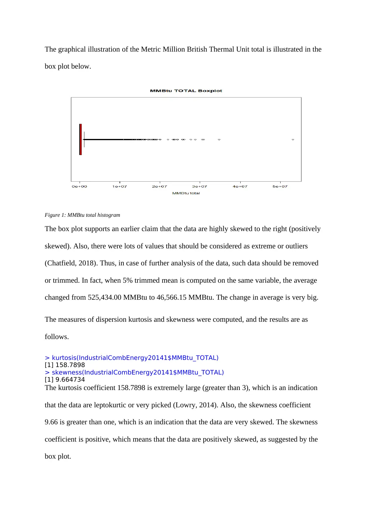
This report presents an analysis of energy consumption data, specifically focusing on the variable MMBtu_TOTAL, using RStudio. The study utilizes data from the Manufacturing Energy Consumption Survey (MECS) to understand energy consumption patterns in US factories. The analysis employs descriptive statistics to examine measures of central tendency (mean, median, and mode) and dispersion (standard deviation, variance, interquartile range, and coefficient of variation). The report highlights the skewed nature of the data, indicating a high concentration of extreme values, which is further supported by graphical illustrations like box plots. The findings reveal a significant difference between the mean and median, indicating positive skewness, along with high kurtosis. The report concludes with a discussion of the implications of these findings and suggests data trimming for further analysis. The R code used for the analysis is provided in the appendix.

RStudio: Interpret the Central Measures of a Variable
Name:
Institution:

Introduction
This report used the Manufacturing Energy Consumption Survey (MECS) except the
Petroleum Refining Industry survey data. The survey covered about 97-98% of the
manufacturing payroll, which implies that the data mirrors the US factories energy
consumption. There were two main assumptions by MECS on the consumption of the energy
are: i) the energy produced was used off one-shot; ii) and the production on-site is consumed
first, then feedstock and lastly the fuel. Probabilistic approach (Stratified probability
proportionate to size PPS) was used to obtain a representative sample of the population
(Keller, 2015).
The variable Metric Million British Thermal Unit total (MMBtu_TOTAL) was analyzed. The
analysis helped us understand the distribution of energy consumption in different factories in
the US. Descriptive analysis helped understand the measures of central tendency as well as
the measures of dispersion.
Method
The quantitative method has been one of the most used mathematical approaches to get
meaningful information from the data. It has been vastly developed and utilized across all
fields that use the data. However, before running complex inferential analysis, one needs to
understand the basic descriptive statistics of the data. In this case, we explore the descriptive
statistics of the data to understand their distribution. In particular, for a normal distribution,
the average and the standard deviation are used to define the whole data distribution. When
the data are heavily skewed, the mean is not a reliable measure of central tendency rather the
researcher should use median. Apart from these crucial statistics, other measures of
dispersion were computed and discussed. First, the mean and standard deviation helped
examine the data distribution, whereas other measures of central tendency and dispersion

helped in identifying the shape of the distribution. For instance, Keller, (2014) indicates that
when the mean is the smallest and the mode the largest among the three measures of central
tendency (mean, median and mode) the data are more likely to be negatively skewed
(Chatfield, 2018). The converse is true. If the mean, mode, and median coincide, then the
data are expected to be normally distributed or to have a bell-shaped plot.
The standard deviation is one of the most used measures of dispersion, but very hard to
interpret on its own. Also, in presence of outliers the standard deviation is inflated. Ideally,
the standard deviation divided by the mean (coefficient of variation (CV)) is mostly used to
express the variability of data relative to its average (Kolaczyk & Csárdi, 2014). Graphical
illustration was used to show data distribution. In particular, box plot, which is commonly
referred to as box and whisker, was used to show the data distribution. The box plot gives a
visual illustration of data, and one can construe whether the data are skewed or not and
whether there are outliers. However, from the plot, one cannot deduce the exact values of
central tendency or measures of dispersion (Chambers, 2017). Also, when the data have a
heavy tail and lots of outliers or extreme values, the box plot becomes distorted and may
sometimes not give a meaningful illustration.
Results
Descriptive analysis for the variable Metric Million British Thermal Unit total
(MMBtu_TOTAL) is carried out and the results are as follows:
> mean(IndustrialCombEnergy20141$MMBtu_TOTAL)
[1] 525434.4
The summary indicates that on average, factories utilizes 525,434.40 Metric Million British
Thermal Unit in the US. This implies that if a factory is randomly selected, it is expected to
consume on average this amount of metric million British thermal units (Keller, 2015).
The median and mode are computed and the results are as follows:

getmode(IndustrialCombEnergy20141$MMBtu_TOTAL)
[1] 876.3664
> median(IndustrialCombEnergy20141$MMBtu_TOTAL)
[1] 46566.15
The summary indicates that the median 46,566.15 MMBtu is significantly lower than the
mean and mode 876.3664 MMBtu is even smaller (Lowry, 2014). This difference implies
that there are a lot of extreme values to the right-hand side of the mean. This inflates the
value of the average. In other words, the MMBtu total data are highly skewed to the right or
positively skewed.
The measures of dispersion are computed and the results are as follows.
var(IndustrialCombEnergy20141$MMBtu_TOTAL)
[1] 2.523967e+12
> sd(IndustrialCombEnergy20141$MMBtu_TOTAL)
[1] 1588700
> summary(IndustrialCombEnergy20141$MMBtu_TOTAL)
Min. 1st Qu. Median Mean 3rd Qu. Max.
1 2015 46566 525434 467936 53099894
The results show that the variance of the MMBtu total in the US is extremely big, which only
means that there were lots of inconsistencies in energy consumption in factories (Sullivan III,
2015). The factories consume a minimum of 1 MMBtu energy total and a maximum of
53,099,894 MMBtu. This implies that the range is 53099893 MMBtu, which is extremely
big. The quartile values suggest that the energy consumption of the middle 50% of the
factories lies between 2015 MMBtu and 467,936 MMBtu. The upper and lower quartile
difference (Interquartile range abbreviated as IQR) is 465921 MMBtu, which paints a better
picture of variability among energy consumption. The IQR is a better measurement of
dispersion than variance (standard deviation), and range as the outliers do not influence it
(Kolaczyk & Csárdi, 2014).
The coefficient of variation (CV) is computed and the results are as follows:
cvMMBtu
[1] 3.02359
The value indicates that the standard deviation is 302.359% times greater than the mean
(Lowry, 2014). This shows that energy consumption was very dispersed.

The graphical illustration of the Metric Million British Thermal Unit total is illustrated in the
box plot below.
Figure 1: MMBtu total histogram
The box plot supports an earlier claim that the data are highly skewed to the right (positively
skewed). Also, there were lots of values that should be considered as extreme or outliers
(Chatfield, 2018). Thus, in case of further analysis of the data, such data should be removed
or trimmed. In fact, when 5% trimmed mean is computed on the same variable, the average
changed from 525,434.00 MMBtu to 46,566.15 MMBtu. The change in average is very big.
The measures of dispersion kurtosis and skewness were computed, and the results are as
follows.
> kurtosis(IndustrialCombEnergy20141$MMBtu_TOTAL)
[1] 158.7898
> skewness(IndustrialCombEnergy20141$MMBtu_TOTAL)
[1] 9.664734
The kurtosis coefficient 158.7898 is extremely large (greater than 3), which is an indication
that the data are leptokurtic or very picked (Lowry, 2014). Also, the skewness coefficient
9.66 is greater than one, which is an indication that the data are very skewed. The skewness
coefficient is positive, which means that the data are positively skewed, as suggested by the
box plot.

References
Chambers, J. M. (2017). Graphical Methods for Data Analysis: 0. Chapman and Hall/CRC.
Chatfield, C. (2018). Statistics for technology: a course in applied statistics (3rd Edition ed.).
New York: Routledge.
Keller, G. (2015). Statistics for Management and Economics, Abbreviated. Cengage
Learning.
Kolaczyk, E. D., & Csárdi, G. (2014). Statistical analysis of network data with R (Vol. 65).
New York: Springer.
Lowry, R. (2014). Concepts and applications of inferential statistics.
Sullivan III, M. (2015). Fundamentals of statistics. Pearson.

Appendix: R-code
##### Central Measures of a Variables and dispersion ####
mean(IndustrialCombEnergy20141$MMBtu_TOTAL)
mean(IndustrialCombEnergy20141$MMBtu_TOTAL,trim=5)
median(IndustrialCombEnergy20141$MMBtu_TOTAL)
#finging the mode
getmode <- function(x) {
uniqv <- unique(x)
uniqv[which.max(tabulate(match(x, uniqv)))]
}
#calling for the mode
getmode(IndustrialCombEnergy20141$MMBtu_TOTAL)
var(IndustrialCombEnergy20141$MMBtu_TOTAL)
sd(IndustrialCombEnergy20141$MMBtu_TOTAL)
summary(IndustrialCombEnergy20141$MMBtu_TOTAL)
max(IndustrialCombEnergy20141$MMBtu_TOTAL)
xbar1=mean(IndustrialCombEnergy20141$MMBtu_TOTAL)
s1=sd(IndustrialCombEnergy20141$MMBtu_TOTAL)
cvMMBtu
boxplot(IndustrialCombEnergy20141$MMBtu_TOTAL,
horizontal = T,
main = "MMBtu TOTAL Boxplot",
col="red",
xlab="MMBtu total")

# measures of spread
install.packages("moments")
library("moments")
kurtosis(IndustrialCombEnergy20141$MMBtu_TOTAL)
skewness(IndustrialCombEnergy20141$MMBtu_TOTAL)