Comprehensive Sales Data Analysis Report: 2002 Australian Orders
VerifiedAdded on 2020/05/28
|16
|2920
|220
Report
AI Summary
This report presents a comprehensive analysis of sales data, focusing on a sample of 60 orders from Australian sales data. The analysis includes summary statistics for quantitative variables such as order quantity, sales, shipping costs, and days to ship, along with graphical representations for qualitative variables like order priority, ship mode, customer type, and region. Statistical tests, including Z-tests and two-sample t-tests, are employed to assess the representativeness of the sample data and compare shipping costs across different order priorities and sales differences between eastern and western regions. The report also explores the relationship between sales and order quantity using correlation and regression techniques to predict sales based on order quantity, providing insights into key business aspects like customer preferences, shipping costs, and regional sales variations. The results show that customers prefer high priority orders and regular Air mode delivery, and the average sales order for the western states and the eastern states are nearly equal.
Executive Summary:
The analysis is based on a sample of 60 American sales data. The results of the analysis
indicates that, the average order quantity for 60 customers is about 24.31 and variations
in average quantity is about 15.14. The customers who buy the products are mostly
belongs to the home office type. The average sales of items is about 1716 and the
customers mostly prefer regular Air mode delivery system to deliver the sales items.
The average shipping cost is the delivery for the customers is about $12.57 and deviation
in the shipping cost form average shipping cost is about $15.93, the customer’s mostly
preferred the eastern region as a delivery space for delivery of selling items and the
average number of days for shipment of sold items is about 1.71. The priority order of
critical type have lower shipping cost comparison to the low priority order type. The average
sales order for the western states and the eastern states are nearly equal, so the customers
who are living in the western state and eastern are not facing problems in the delivery
space.
Paraphrase This Document
Need a fresh take? Get an instant paraphrase of this document with our AI Paraphraser
Introduction:
The analysis is based on the Australian Sales data of 2002 orders. It is mentioned that to
select the sample of 60 observations from Australian Sales data use the random number
table. The purpose of the report based on the summary statistics of quantitative variables
and graphical representation of the all qualitative variables. The report includes the
followings:
1. Whether average sale amount order for home office customers for sample orders is a
representative of population average sales orders.
2. Whether the sample average shipping cost for sample orders represents the population
average shipping costs.
3. Whether the critical priority order would have higher shipping costs than low priority
order.
4. Is the average sales order are different for Eastern and Western regions?
5. It also includes the prediction of sales by using the order quantity.
Use Z-test to do the analysis whether the amount of orders for average sales in sample of
home office customers represents the amount of orders for population average sales for
home office customers, and whether sample average shipping costs for all sample orders
represents the population average shipping costs for all sample orders.
Use two sample independent t -test, to do the analysis that the critical priority order
would have higher shipping costs comparison to the low priority order, and whether the
mean sale orders are different for Eastern and Western regions.
The correlation technique will be used to know about the relationship between sales and
order quantity, and to predict the sales by using order quantity, the regression technique
will be used.
Analysis:
To select a random sample of size 60 from the 2002 orders, use random number table.
The random number table includes the values in a random order, so to get the sample of
size 60 from the 2002 orders, select only that random numbers which are less than 2002
and skip the other numbers. Thus, the 60 order numbers will be observed form the table
which are less than 2002. Now, write the data of selected 60 numbers from Australian
Sales into a new excel sheet. The sample of 60 orders will be generated.
Now use the sample data to calculate the summary statistics for quantitative variables and
to draw the graphical summary for the qualitative variables. The summary statistics for
each of the variable is given below:
1. Order priority indicates importance of order, the value indicates a Critical order, the
value 3 indicates a high order, the value 2 indicates a medium order, the value 1indicates
a low order and the value 0 indicates a not specified order. So the variable order priority
is a qualitative variable. The frequency of each variable and the bar graph is shown
below:
Variable\Statistic Nbr. of
observations
Nbr. of
categories
Mode
frequency
Categories Frequency
per
category
Order Priority 60 5 16 0 16.00
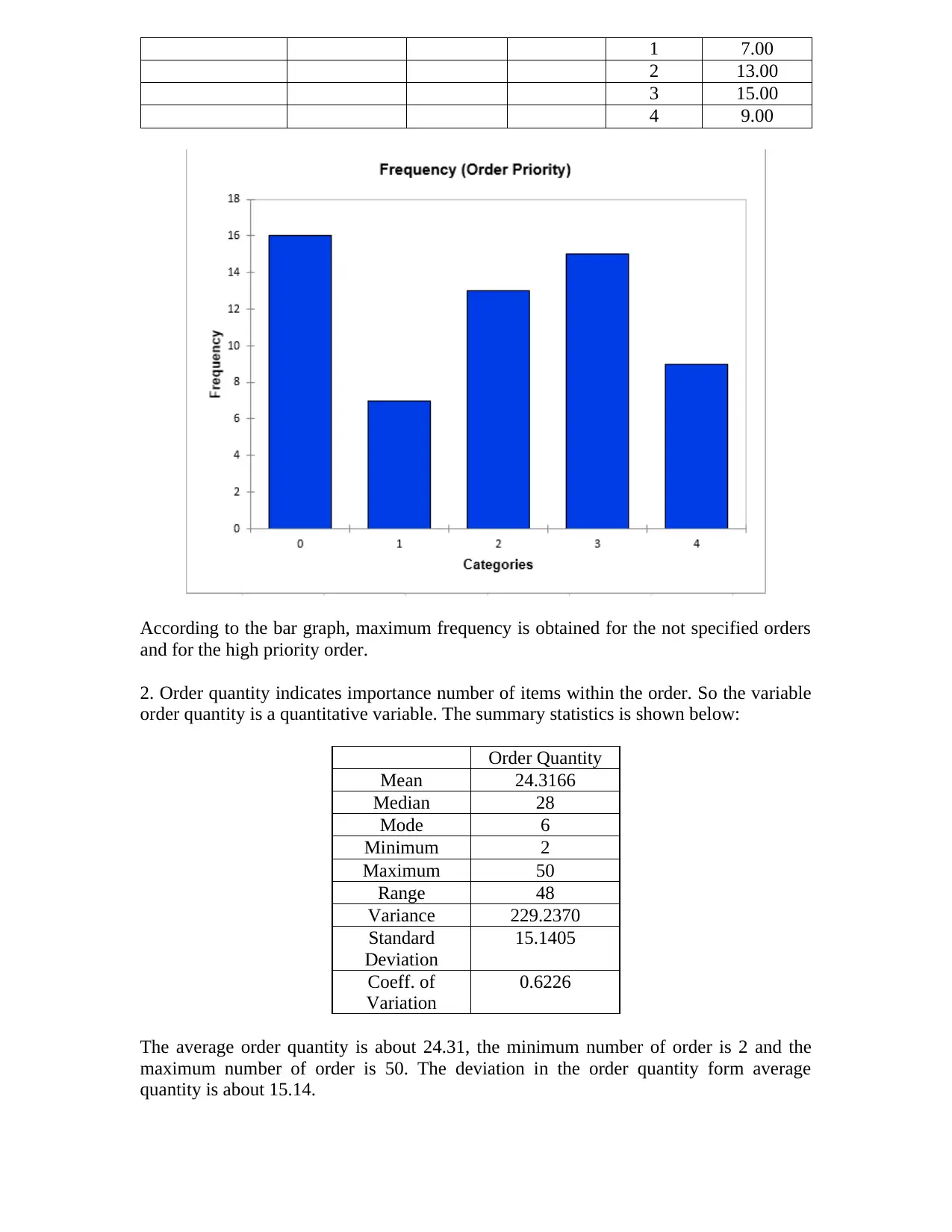
1 7.00
2 13.00
3 15.00
4 9.00
According to the bar graph, maximum frequency is obtained for the not specified orders
and for the high priority order.
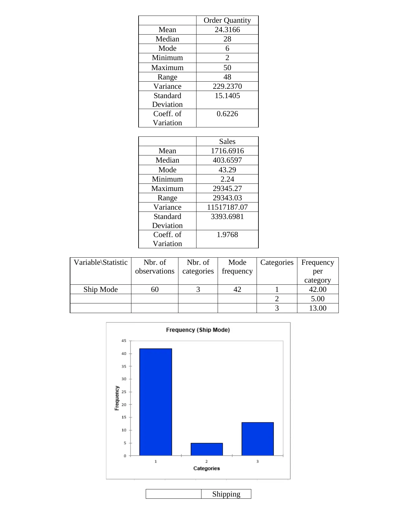
2. Order quantity indicates importance number of items within the order. So the variable
order quantity is a quantitative variable. The summary statistics is shown below:
Order Quantity
Mean 24.3166
Median 28
Mode 6
Minimum 2
Maximum 50
Range 48
Variance 229.2370
Standard
Deviation
15.1405
Coeff. of
Variation
0.6226
The average order quantity is about 24.31, the minimum number of order is 2 and the
maximum number of order is 50. The deviation in the order quantity form average
quantity is about 15.14.
2 13.00
3 15.00
4 9.00
According to the bar graph, maximum frequency is obtained for the not specified orders
and for the high priority order.
2. Order quantity indicates importance number of items within the order. So the variable
order quantity is a quantitative variable. The summary statistics is shown below:
Order Quantity
Mean 24.3166
Median 28
Mode 6
Minimum 2
Maximum 50
Range 48
Variance 229.2370
Standard
Deviation
15.1405
Coeff. of
Variation
0.6226
The average order quantity is about 24.31, the minimum number of order is 2 and the
maximum number of order is 50. The deviation in the order quantity form average
quantity is about 15.14.
⊘ This is a preview!⊘
Do you want full access?
Subscribe today to unlock all pages.
Trusted by 1+ million students worldwide
3. Sales indicates sales of items. So the variable sales is a quantitative variable. The
summary statistics is shown below:
Sales
Mean 1716.6916
Median 403.6597
Mode 43.29
Minimum 2.24
Maximum 29345.27
Range 29343.03
Variance 11517187.07
Standard
Deviation
3393.6981
Coeff. of
Variation
1.9768
The average sales is about 1716, the minimum number of sales is 2 and the maximum
number of sales is 29435. The deviation in the sales form average sales is about 3393.
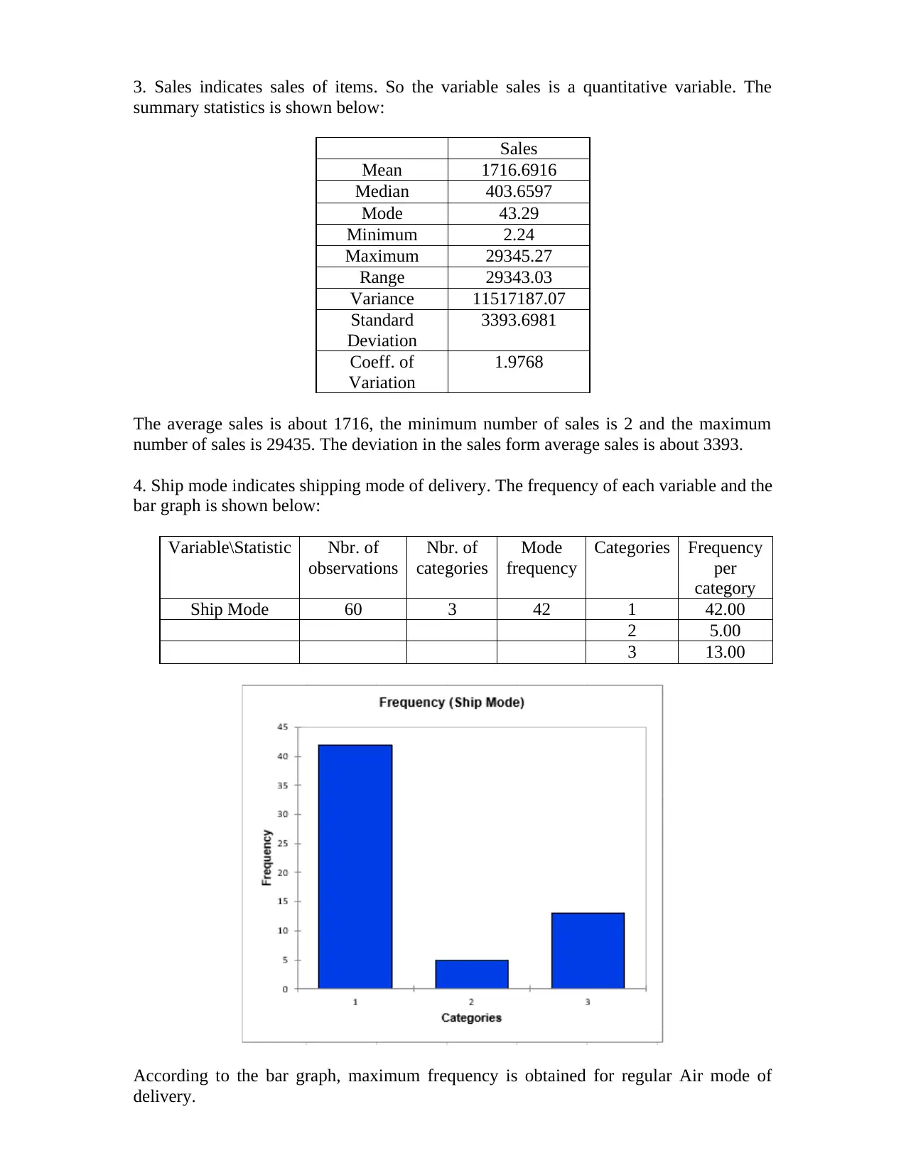
4. Ship mode indicates shipping mode of delivery. The frequency of each variable and the
bar graph is shown below:
Variable\Statistic Nbr. of
observations
Nbr. of
categories
Mode
frequency
Categories Frequency
per
category
Ship Mode 60 3 42 1 42.00
2 5.00
3 13.00
According to the bar graph, maximum frequency is obtained for regular Air mode of
delivery.
summary statistics is shown below:
Sales
Mean 1716.6916
Median 403.6597
Mode 43.29
Minimum 2.24
Maximum 29345.27
Range 29343.03
Variance 11517187.07
Standard
Deviation
3393.6981
Coeff. of
Variation
1.9768
The average sales is about 1716, the minimum number of sales is 2 and the maximum
number of sales is 29435. The deviation in the sales form average sales is about 3393.
4. Ship mode indicates shipping mode of delivery. The frequency of each variable and the
bar graph is shown below:
Variable\Statistic Nbr. of
observations
Nbr. of
categories
Mode
frequency
Categories Frequency
per
category
Ship Mode 60 3 42 1 42.00
2 5.00
3 13.00
According to the bar graph, maximum frequency is obtained for regular Air mode of
delivery.
Paraphrase This Document
Need a fresh take? Get an instant paraphrase of this document with our AI Paraphraser
5. Shipping Cost indicates the total dollar amount of shipping cost. So the variable
shipping cost is a quantitative variable. The summary statistics is shown below:
Shipping
Cost
Mean 12.5713
Median 6.635
Mode 19.99
Minimum 0.5
Maximum 99
Range 98.5
Variance 253.8996
Standard
Deviation
15.9342
Coeff. of
Variation
1.2675
The average shipping cost is about $12.57, the minimum number shipping cost is $0.5
and the maximum shipping cost is $99. The deviation in the shipping cost form average
shipping cost is about $15.93.
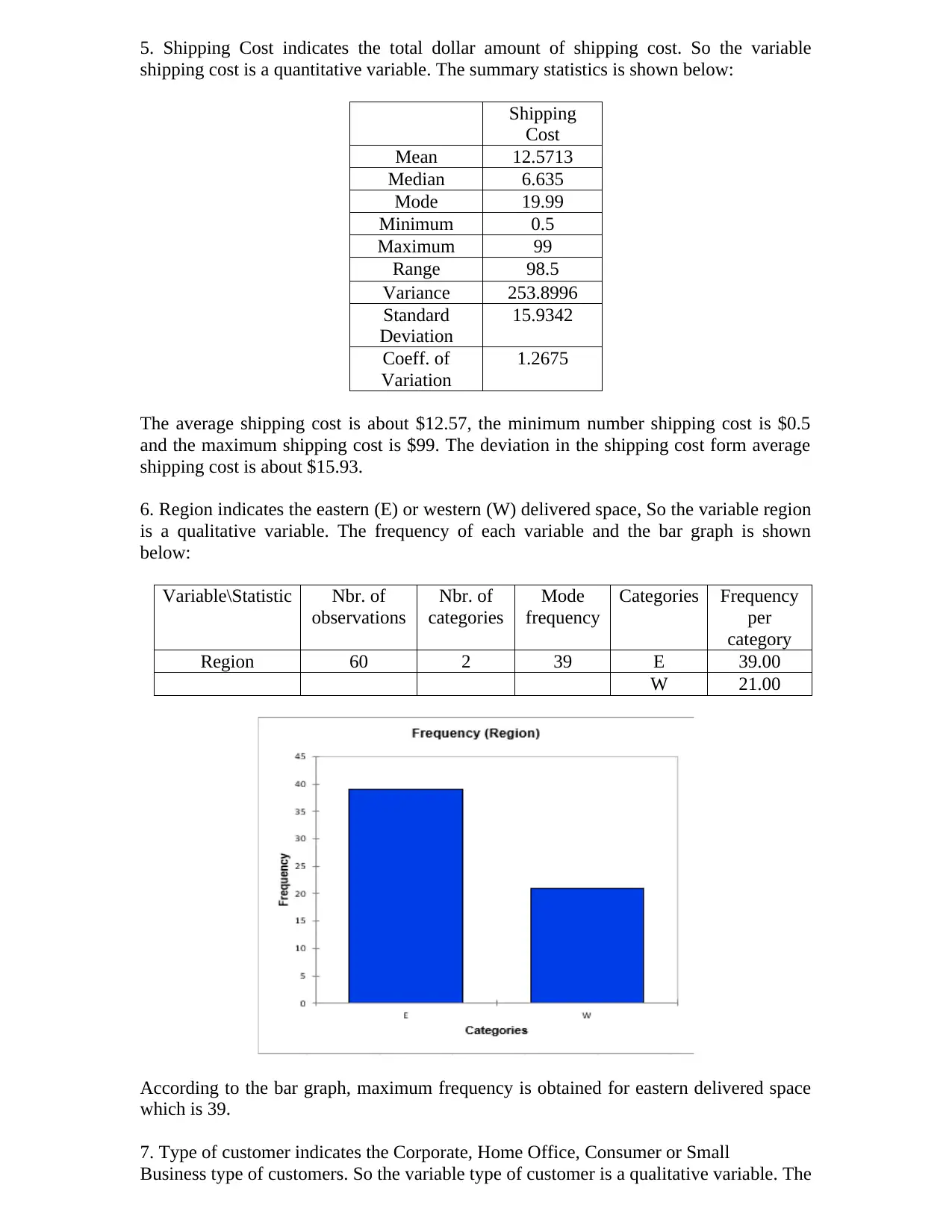
6. Region indicates the eastern (E) or western (W) delivered space, So the variable region
is a qualitative variable. The frequency of each variable and the bar graph is shown
below:
Variable\Statistic Nbr. of
observations
Nbr. of
categories
Mode
frequency
Categories Frequency
per
category
Region 60 2 39 E 39.00
W 21.00
According to the bar graph, maximum frequency is obtained for eastern delivered space
which is 39.
7. Type of customer indicates the Corporate, Home Office, Consumer or Small
Business type of customers. So the variable type of customer is a qualitative variable. The
shipping cost is a quantitative variable. The summary statistics is shown below:
Shipping
Cost
Mean 12.5713
Median 6.635
Mode 19.99
Minimum 0.5
Maximum 99
Range 98.5
Variance 253.8996
Standard
Deviation
15.9342
Coeff. of
Variation
1.2675
The average shipping cost is about $12.57, the minimum number shipping cost is $0.5
and the maximum shipping cost is $99. The deviation in the shipping cost form average
shipping cost is about $15.93.
6. Region indicates the eastern (E) or western (W) delivered space, So the variable region
is a qualitative variable. The frequency of each variable and the bar graph is shown
below:
Variable\Statistic Nbr. of
observations
Nbr. of
categories
Mode
frequency
Categories Frequency
per
category
Region 60 2 39 E 39.00
W 21.00
According to the bar graph, maximum frequency is obtained for eastern delivered space
which is 39.
7. Type of customer indicates the Corporate, Home Office, Consumer or Small
Business type of customers. So the variable type of customer is a qualitative variable. The
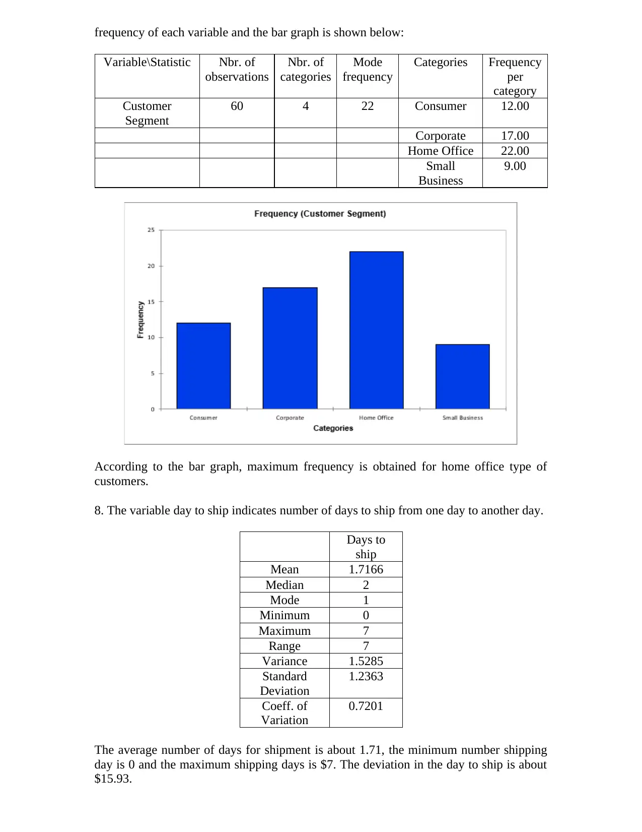
frequency of each variable and the bar graph is shown below:
Variable\Statistic Nbr. of
observations
Nbr. of
categories
Mode
frequency
Categories Frequency
per
category
Customer
Segment
60 4 22 Consumer 12.00
Corporate 17.00
Home Office 22.00
Small
Business
9.00
According to the bar graph, maximum frequency is obtained for home office type of
customers.
8. The variable day to ship indicates number of days to ship from one day to another day.
Days to
ship
Mean 1.7166
Median 2
Mode 1
Minimum 0
Maximum 7
Range 7
Variance 1.5285
Standard
Deviation
1.2363
Coeff. of
Variation
0.7201
The average number of days for shipment is about 1.71, the minimum number shipping
day is 0 and the maximum shipping days is $7. The deviation in the day to ship is about
$15.93.
⊘ This is a preview!⊘
Do you want full access?
Subscribe today to unlock all pages.
Trusted by 1+ million students worldwide
The confidence interval for amount of average sales for home office customers is:
Statistic Sales | Home Office
Lower bound on mean (95%) 307.8443
Upper bound on mean (95%) 5175.6964
And the actual population mean for the home office customers is:
Statistic Sales | Home Office
Nbr. of observations 497
Mean 1585.0821
So, the 95% confidence interval is (307. 84, 5175.69), So we are 95% confidence that the
actual population mean for the home office customers will lies within the 95%
confidence interval for the sample data of home office customers.
The 95% confidence interval for average shipping costs for all sample orders is:
Statistic Shipping Cost
Lower bound on mean
(95%)
8.4550
Upper bound on mean (95%) 16.6875
And the actual population mean for average shipping costs is:
Statistic Shipping Cost
Nbr. of observations 2002
Mean 12.4501
So, the 95% confidence interval for the average shipping costs for all is (8.45, 16.68), So
we are 95% confidence that the actual population mean for average shipping costs will
lies within the 95% confidence interval for the sample data average shipping costs.
To test that the shipping cost for critical priority order is greater than shipping of an order
of low priority, use two sample t-test. The results for 2 sample t-test is shown below:
t-Test: Two-Sample Assuming Unequal Variances
Shipping Cost
(Critical)
Shipping Cost
(Low)
Mean 13.7089 8.1871
Variance 355.2823 39.6037
Observations 9 7
Hypothesized Mean
Difference
0
df 10
t Stat 0.8219
P(T<=t) one-tail 0.2151
t Critical one-tail 1.8124
P(T<=t) two-tail 0.4303
t Critical two-tail 2.2281
Statistic Sales | Home Office
Lower bound on mean (95%) 307.8443
Upper bound on mean (95%) 5175.6964
And the actual population mean for the home office customers is:
Statistic Sales | Home Office
Nbr. of observations 497
Mean 1585.0821
So, the 95% confidence interval is (307. 84, 5175.69), So we are 95% confidence that the
actual population mean for the home office customers will lies within the 95%
confidence interval for the sample data of home office customers.
The 95% confidence interval for average shipping costs for all sample orders is:
Statistic Shipping Cost
Lower bound on mean
(95%)
8.4550
Upper bound on mean (95%) 16.6875
And the actual population mean for average shipping costs is:
Statistic Shipping Cost
Nbr. of observations 2002
Mean 12.4501
So, the 95% confidence interval for the average shipping costs for all is (8.45, 16.68), So
we are 95% confidence that the actual population mean for average shipping costs will
lies within the 95% confidence interval for the sample data average shipping costs.
To test that the shipping cost for critical priority order is greater than shipping of an order
of low priority, use two sample t-test. The results for 2 sample t-test is shown below:
t-Test: Two-Sample Assuming Unequal Variances
Shipping Cost
(Critical)
Shipping Cost
(Low)
Mean 13.7089 8.1871
Variance 355.2823 39.6037
Observations 9 7
Hypothesized Mean
Difference
0
df 10
t Stat 0.8219
P(T<=t) one-tail 0.2151
t Critical one-tail 1.8124
P(T<=t) two-tail 0.4303
t Critical two-tail 2.2281
Paraphrase This Document
Need a fresh take? Get an instant paraphrase of this document with our AI Paraphraser
The value of the t-Statistic is 0.821 and the corresponding P-Value at 10 degree of
freedom for one tail test is 0.215. Now compare P-value with the level of significance
(0.05), the P-Value is greater than the level of significance (0.05), so the null hypothesis
of the test does not get rejected. Hence there is insignificance evidence to conclude that
shipping cost for critical priority order is greater than shipping of an order of low priority.
To test average sales order are different in the eastern and western, use two sample t-test.
The results for 2 sample t-test is shown below:
t-Test: Two-Sample Assuming Unequal Variances
Sales (WES) Sales (EAS)
Mean 1371.6728 2917.5313
Variance 15652257.89 23360582.44
Observations 21 39
Hypothesized Mean
Difference
0
df 49
t Stat -1.3332
P(T<=t) one-tail 0.0943
t Critical one-tail 1.6765
P(T<=t) two-tail 0.1886
t Critical two-tail 2.0095
The value of the t-Statistic is 1.33 and the corresponding P-Value at 49 degree of
freedom for two tailed test is 0.188. Now compare P-value with the level of significance
(0.05), the P-Value is larger than the level of significance (0.05), so the null hypothesis of
the test does not get rejected. Hence there is insignificance evidence to conclude that
average sales order are different in the eastern and western states.
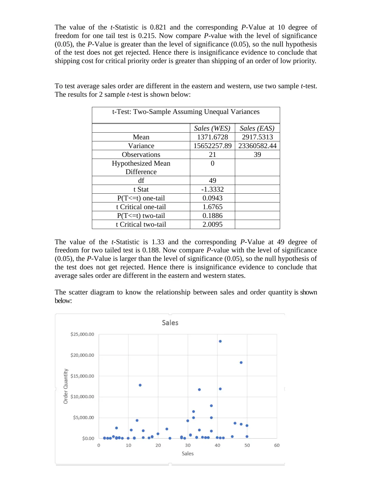
The scatter diagram to know the relationship between sales and order quantity is shown
below:
freedom for one tail test is 0.215. Now compare P-value with the level of significance
(0.05), the P-Value is greater than the level of significance (0.05), so the null hypothesis
of the test does not get rejected. Hence there is insignificance evidence to conclude that
shipping cost for critical priority order is greater than shipping of an order of low priority.
To test average sales order are different in the eastern and western, use two sample t-test.
The results for 2 sample t-test is shown below:
t-Test: Two-Sample Assuming Unequal Variances
Sales (WES) Sales (EAS)
Mean 1371.6728 2917.5313
Variance 15652257.89 23360582.44
Observations 21 39
Hypothesized Mean
Difference
0
df 49
t Stat -1.3332
P(T<=t) one-tail 0.0943
t Critical one-tail 1.6765
P(T<=t) two-tail 0.1886
t Critical two-tail 2.0095
The value of the t-Statistic is 1.33 and the corresponding P-Value at 49 degree of
freedom for two tailed test is 0.188. Now compare P-value with the level of significance
(0.05), the P-Value is larger than the level of significance (0.05), so the null hypothesis of
the test does not get rejected. Hence there is insignificance evidence to conclude that
average sales order are different in the eastern and western states.
The scatter diagram to know the relationship between sales and order quantity is shown
below:
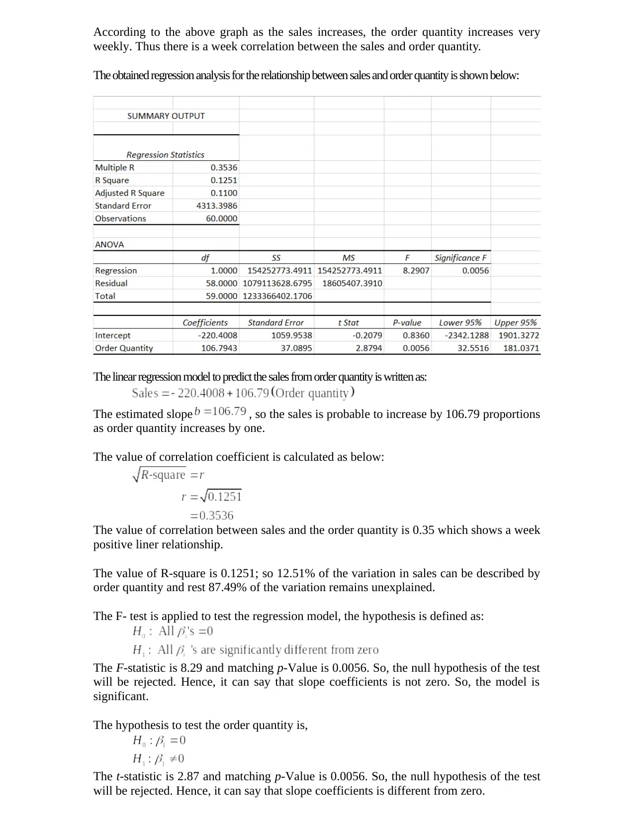
According to the above graph as the sales increases, the order quantity increases very
weekly. Thus there is a week correlation between the sales and order quantity.
The obtained regression analysis for the relationship between sales and order quantity is shown below:
The linear regression model to predict the sales from order quantity is written as:
The estimated slope , so the sales is probable to increase by 106.79 proportions
as order quantity increases by one.
The value of correlation coefficient is calculated as below:
The value of correlation between sales and the order quantity is 0.35 which shows a week
positive liner relationship.
The value of R-square is 0.1251; so 12.51% of the variation in sales can be described by
order quantity and rest 87.49% of the variation remains unexplained.
The F- test is applied to test the regression model, the hypothesis is defined as:
The F-statistic is 8.29 and matching p-Value is 0.0056. So, the null hypothesis of the test
will be rejected. Hence, it can say that slope coefficients is not zero. So, the model is
significant.
The hypothesis to test the order quantity is,
The t-statistic is 2.87 and matching p-Value is 0.0056. So, the null hypothesis of the test
will be rejected. Hence, it can say that slope coefficients is different from zero.
⊘ This is a preview!⊘
Do you want full access?
Subscribe today to unlock all pages.
Trusted by 1+ million students worldwide
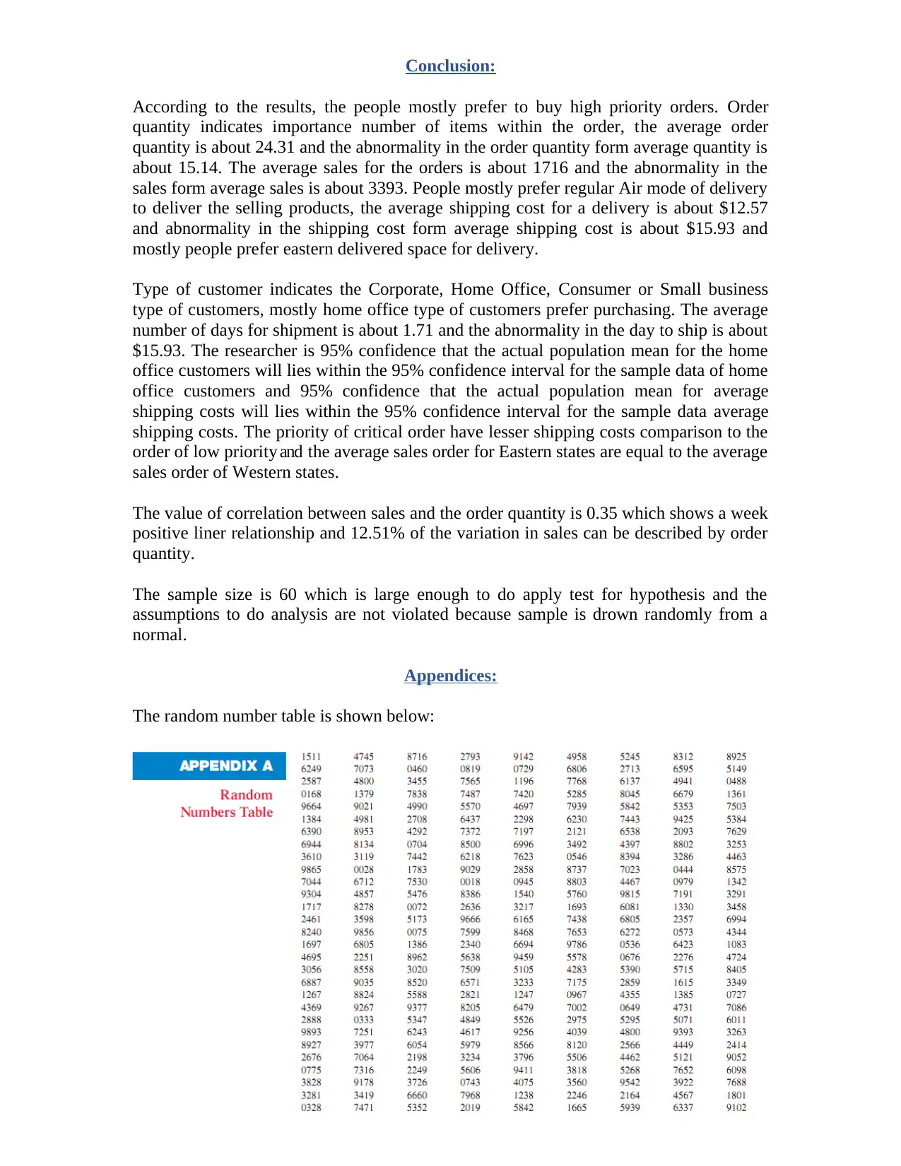
Conclusion:
According to the results, the people mostly prefer to buy high priority orders. Order
quantity indicates importance number of items within the order, the average order
quantity is about 24.31 and the abnormality in the order quantity form average quantity is
about 15.14. The average sales for the orders is about 1716 and the abnormality in the
sales form average sales is about 3393. People mostly prefer regular Air mode of delivery
to deliver the selling products, the average shipping cost for a delivery is about $12.57
and abnormality in the shipping cost form average shipping cost is about $15.93 and
mostly people prefer eastern delivered space for delivery.
Type of customer indicates the Corporate, Home Office, Consumer or Small business
type of customers, mostly home office type of customers prefer purchasing. The average
number of days for shipment is about 1.71 and the abnormality in the day to ship is about
$15.93. The researcher is 95% confidence that the actual population mean for the home
office customers will lies within the 95% confidence interval for the sample data of home
office customers and 95% confidence that the actual population mean for average
shipping costs will lies within the 95% confidence interval for the sample data average
shipping costs. The priority of critical order have lesser shipping costs comparison to the
order of low priority and the average sales order for Eastern states are equal to the average
sales order of Western states.
The value of correlation between sales and the order quantity is 0.35 which shows a week
positive liner relationship and 12.51% of the variation in sales can be described by order
quantity.
The sample size is 60 which is large enough to do apply test for hypothesis and the
assumptions to do analysis are not violated because sample is drown randomly from a
normal.
Appendices:
The random number table is shown below:
Paraphrase This Document
Need a fresh take? Get an instant paraphrase of this document with our AI Paraphraser
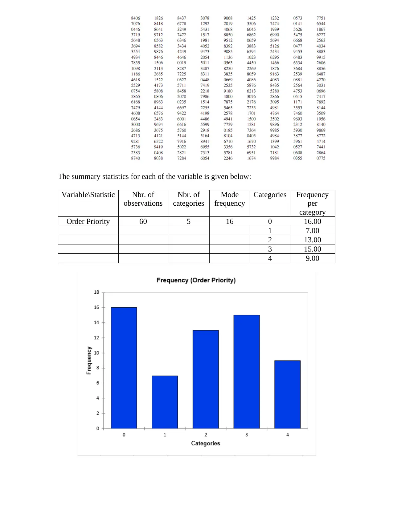
The summary statistics for each of the variable is given below:
Variable\Statistic Nbr. of
observations
Nbr. of
categories
Mode
frequency
Categories Frequency
per
category
Order Priority 60 5 16 0 16.00
1 7.00
2 13.00
3 15.00
4 9.00
Variable\Statistic Nbr. of
observations
Nbr. of
categories
Mode
frequency
Categories Frequency
per
category
Order Priority 60 5 16 0 16.00
1 7.00
2 13.00
3 15.00
4 9.00
Order Quantity
Mean 24.3166
Median 28
Mode 6
Minimum 2
Maximum 50
Range 48
Variance 229.2370
Standard
Deviation
15.1405
Coeff. of
Variation
0.6226
Sales
Mean 1716.6916
Median 403.6597
Mode 43.29
Minimum 2.24
Maximum 29345.27
Range 29343.03
Variance 11517187.07
Standard
Deviation
3393.6981
Coeff. of
Variation
1.9768
Variable\Statistic Nbr. of
observations
Nbr. of
categories
Mode
frequency
Categories Frequency
per
category
Ship Mode 60 3 42 1 42.00
2 5.00
3 13.00
Shipping
⊘ This is a preview!⊘
Do you want full access?
Subscribe today to unlock all pages.
Trusted by 1+ million students worldwide
1 out of 16
Related Documents


Your All-in-One AI-Powered Toolkit for Academic Success.
+13062052269
info@desklib.com
Available 24*7 on WhatsApp / Email
![[object Object]](/_next/static/media/star-bottom.7253800d.svg)
Unlock your academic potential
Copyright © 2020–2026 A2Z Services. All Rights Reserved. Developed and managed by ZUCOL.