Hardware and Garden Supplies: Sales Data Analysis and Insights Report

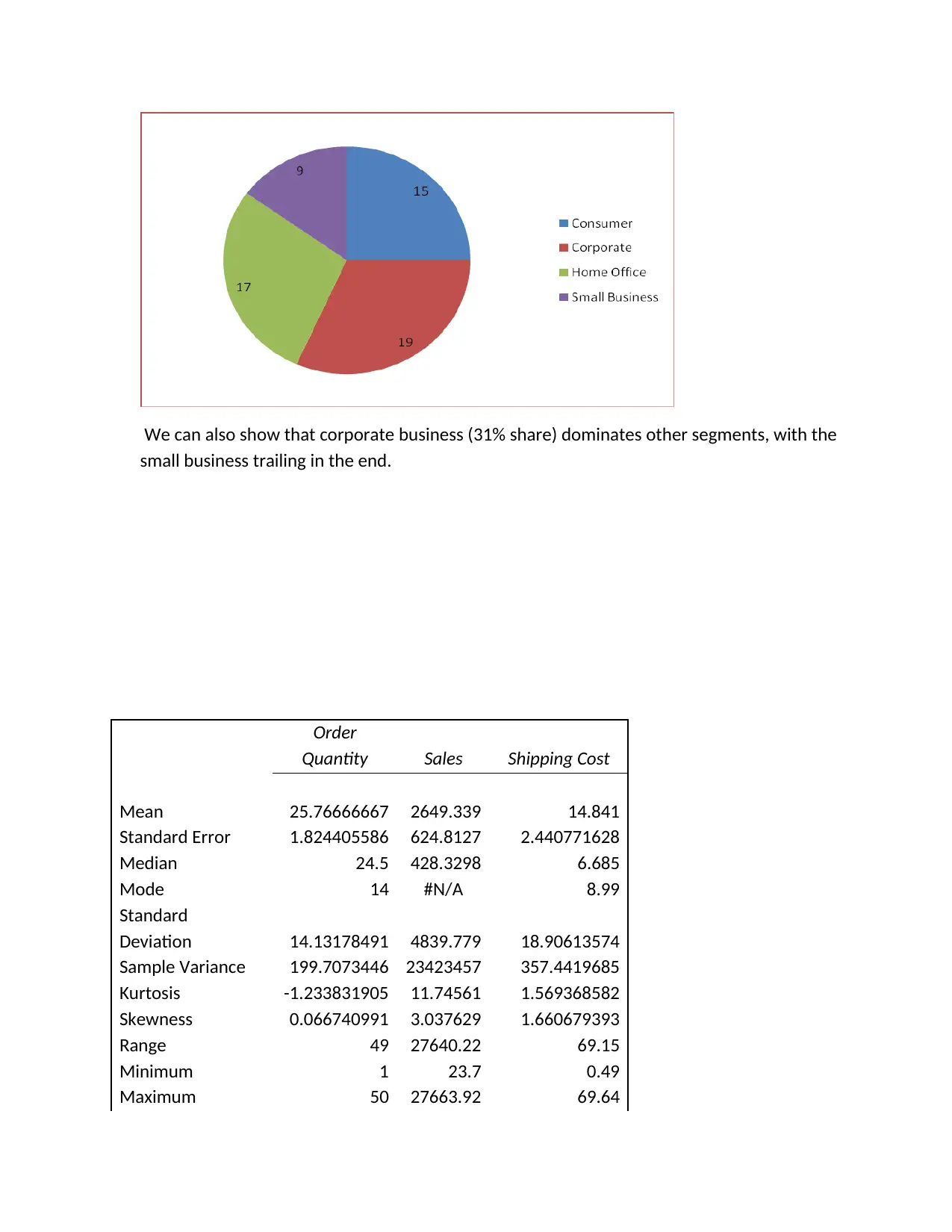
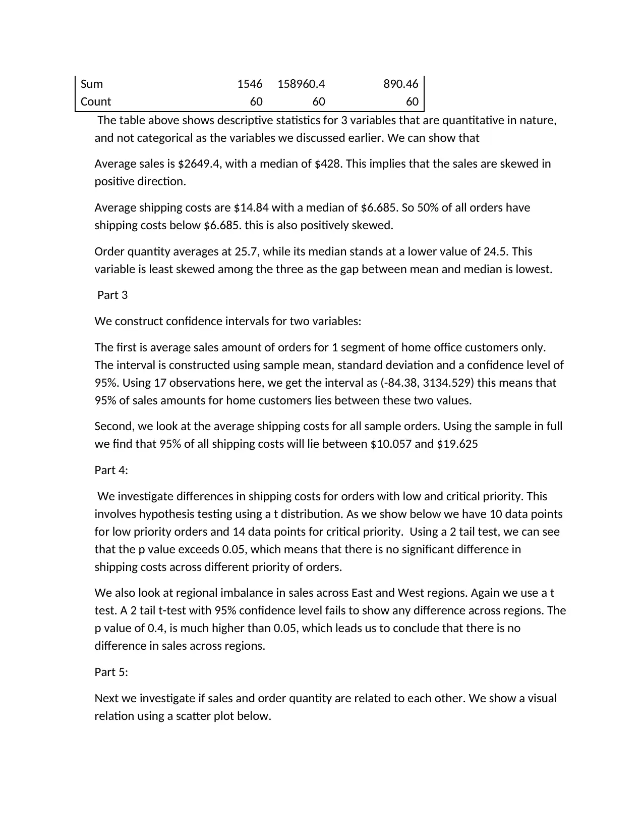
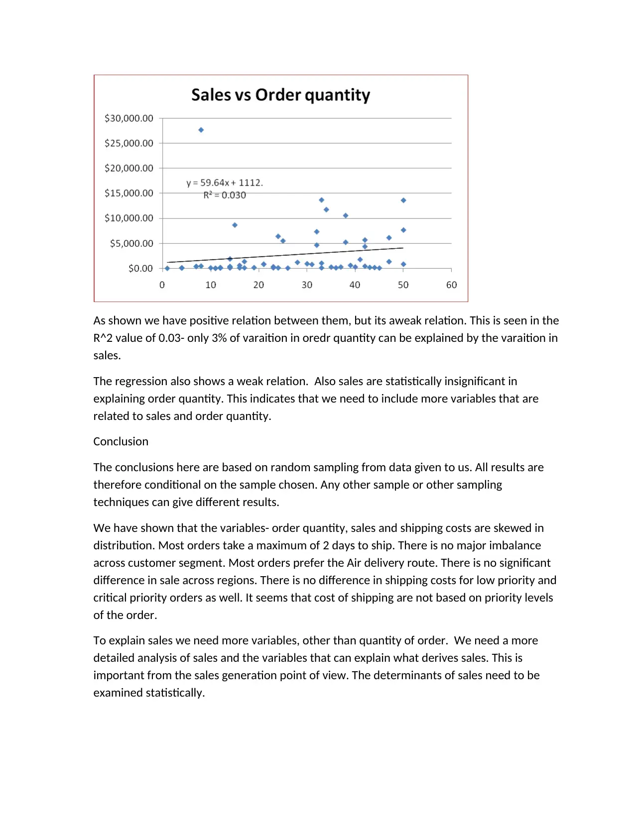
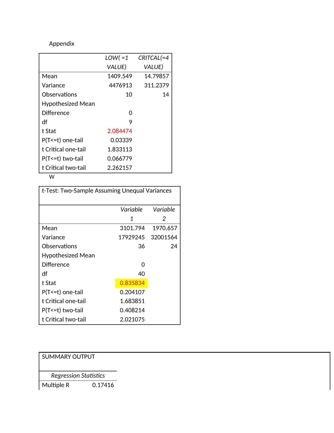
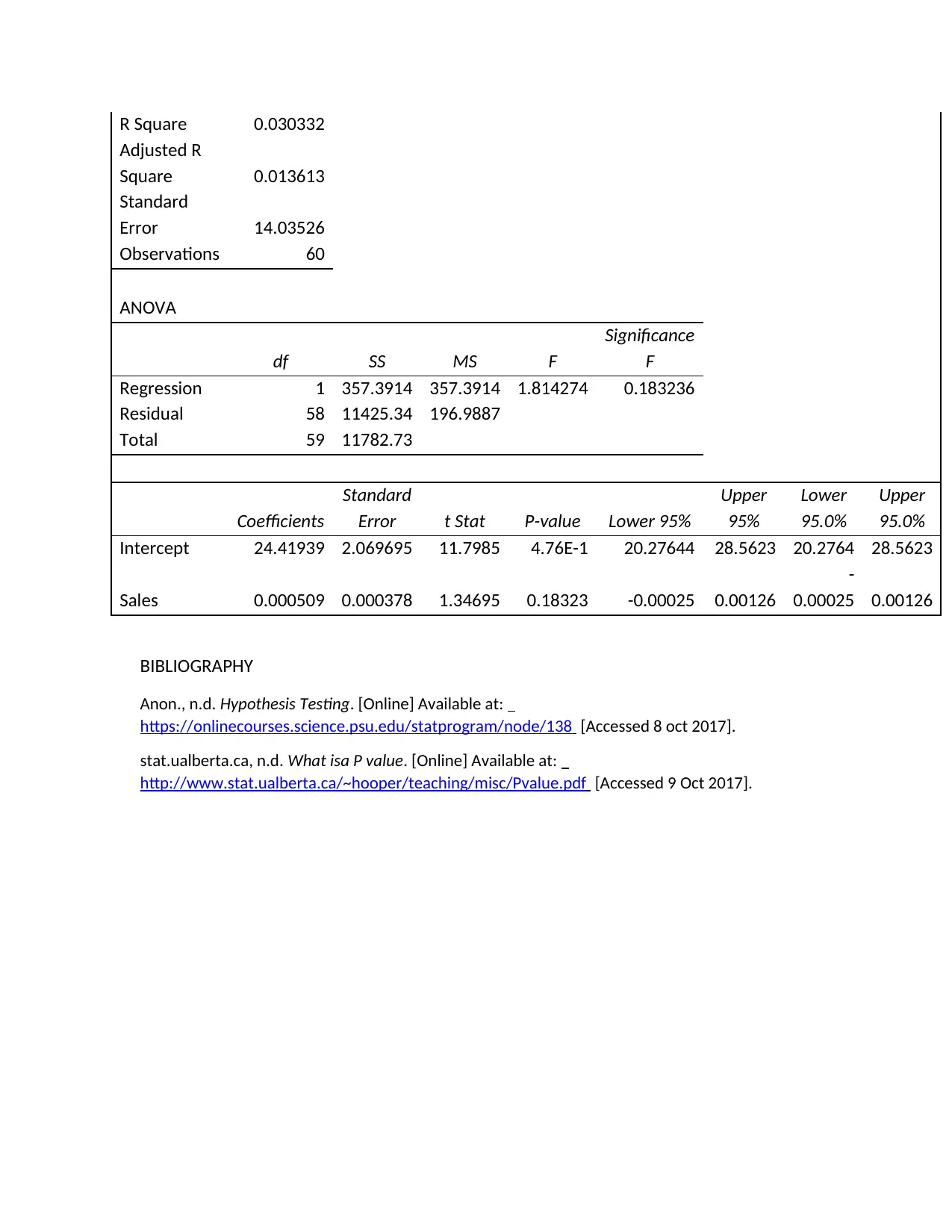
This report presents an analysis of sales data from Hardware and Garden Supplies, based on a random sample of 60 orders. The analysis explores various aspects of the data, including order quantities, sales figures, shipping costs, and customer segments. Statistical methods such as measures of central tendency, dispersion, confidence intervals, hypothesis testing, and regression are employed to derive insights. Key findings include the positive skew of sales and shipping costs, the preferred use of air shipping, and the lack of significant differences in sales across regions or shipping costs for different order priorities. The report also investigates the relationship between sales and order quantity, revealing a weak correlation. The conclusion emphasizes the limitations of the sample and the need for further investigation to understand the determinants of sales. The report provides descriptive statistics, confidence intervals, and the results of hypothesis tests and regression analysis to support its conclusions. The analysis aims to provide a comprehensive overview of the sales data and identify areas for potential improvement and further research.

Executive Summary
We use random sampling to get 60 observation on number of parameters pertaining to
orders of Hardware and Garden Supplies. We can use this data to answer various questions
as mentioned below, along with answers that this report finds
What determines sales? It is clear that order quantity is a poor predictor of sales.
Are orders focused on a particular region? No there is no difference in sales across East and
West.
Do critical orders need higher shipping costs? Again we find no such differences in costs for
orders with different levels of criticality.
Estimates of shipping cost so that customers can be provided with a rough idea about costs.
We show that 95% of all orders will incur shipping costs between $10.057 and $19.625
Average Sales for a particular segment. We show this for Home segment only.
Is a particular shipping mode preferred, which can be targeted in advertisements and by
the sales team? We find that air route is most preferred based on actual data.
How is other data like sales spread? Does this company get most orders of high value or
low value? We find that sales are skewed positively which means that most orders are of
lower value. 50% of orders are of less than $428.
Shipping costs are also skewed, so that 50% of these are below $6.685. Average costs are
higher at $14.8, showing scope for lowering them to control costs and boost profits.
Order quantities average at 25.7, with 50% of orders below 24.5.

Introduction
This report looks at a sample of office supply sales, provided by the ‘Hardware and Garden
Supplies’. We use a sample of 60 out of 20002 data entries given to us pertaining to
different information captured through - order priority and quantity, shipping mode( regular
air/delivery truck/express air), shipping cost, region (East /west), consumer segment
(Corporate/ Home Office/ Consumer/Small Business) and number of days taken to ship the
order. We use this set to derive a sample of 60 observations based on random sampling
technique.
We use Excel to answer a variety of questions pertaining to this data. We use concepts like
measures of central tendency, dispersion, correlation, confidence intervals , hypothesis
testing, regression. We use visual charts that include pie chart, bar chart, scatterplot, and
pivot charts to aid in our analysis. Using Excel tools and statistical concepts we can
understand the distribution of quantitative data like shipping cost, sales, and order quantity.
We can check the share of orders in terms of priority, share of different shipping modes,
customer profile and the average days taken to ship an order. We also look into relation
between sales and order quantity, along with differences in orders with respect o priority
and customer segment. The regional imbalance in orders across East and West is also under
lens here.
Analysis
We divide this section into 5 parts , each of which deals with a separate question and
statistical tool.
Part 1:
We use the RAND function to derive a random number for each of the 2002 points given in
dataset. These are then arranged in ascending order based on the random number allotted
to each. The first 60 data points are taken as the sample set in this report.
Here is a snapshot of the first 5 datapoints in the sample chosen.
Order
Priority
Order
Quantity Sales
Ship
Mode
Shipping
Cost Region
Customer
Segment
Days
to ship
1 45 $75.39 1 $0.70 W Corporate 4
3 42 $451.32 1 $5.16 E Corporate 0
2 39 $616.50 1 $8.40 E
Small
Business 1
0 24
$6,408.3
0 2 $35.67 E Consumer 1

4 42
$4,373.8
5 3 $7.69 E Corporate 1
Part 2:
We now show descriptive statistics for a few variables.
West region dominate sour sample with 36/60 data points for this region.
Most orders ( 74%) are for regular air delivery( = 1on the scale) .

Most orders take 2 days to ship once they are ordered. The majority take 2 or less days as
seen in the chart above.
There is relative equal distribution across priority of different orders.

We can also show that corporate business (31% share) dominates other segments, with the
small business trailing in the end.
Order
Quantity Sales Shipping Cost
Mean 25.76666667 2649.339 14.841
Standard Error 1.824405586 624.8127 2.440771628
Median 24.5 428.3298 6.685
Mode 14 #N/A 8.99
Standard
Deviation 14.13178491 4839.779 18.90613574
Sample Variance 199.7073446 23423457 357.4419685
Kurtosis -1.233831905 11.74561 1.569368582
Skewness 0.066740991 3.037629 1.660679393
Range 49 27640.22 69.15
Minimum 1 23.7 0.49
Maximum 50 27663.92 69.64

Sum 1546 158960.4 890.46
Count 60 60 60
The table above shows descriptive statistics for 3 variables that are quantitative in nature,
and not categorical as the variables we discussed earlier. We can show that
Average sales is $2649.4, with a median of $428. This implies that the sales are skewed in
positive direction.
Average shipping costs are $14.84 with a median of $6.685. So 50% of all orders have
shipping costs below $6.685. this is also positively skewed.
Order quantity averages at 25.7, while its median stands at a lower value of 24.5. This
variable is least skewed among the three as the gap between mean and median is lowest.
Part 3
We construct confidence intervals for two variables:
The first is average sales amount of orders for 1 segment of home office customers only.
The interval is constructed using sample mean, standard deviation and a confidence level of
95%. Using 17 observations here, we get the interval as (-84.38, 3134.529) this means that
95% of sales amounts for home customers lies between these two values.
Second, we look at the average shipping costs for all sample orders. Using the sample in full
we find that 95% of all shipping costs will lie between $10.057 and $19.625
Part 4:
We investigate differences in shipping costs for orders with low and critical priority. This
involves hypothesis testing using a t distribution. As we show below we have 10 data points
for low priority orders and 14 data points for critical priority. Using a 2 tail test, we can see
that the p value exceeds 0.05, which means that there is no significant difference in
shipping costs across different priority of orders.
We also look at regional imbalance in sales across East and West regions. Again we use a t
test. A 2 tail t-test with 95% confidence level fails to show any difference across regions. The
p value of 0.4, is much higher than 0.05, which leads us to conclude that there is no
difference in sales across regions.
Part 5:
Next we investigate if sales and order quantity are related to each other. We show a visual
relation using a scatter plot below.

As shown we have positive relation between them, but its aweak relation. This is seen in the
R^2 value of 0.03- only 3% of varaition in oredr quantity can be explained by the varaition in
sales.
The regression also shows a weak relation. Also sales are statistically insignificant in
explaining order quantity. This indicates that we need to include more variables that are
related to sales and order quantity.
Conclusion
The conclusions here are based on random sampling from data given to us. All results are
therefore conditional on the sample chosen. Any other sample or other sampling
techniques can give different results.
We have shown that the variables- order quantity, sales and shipping costs are skewed in
distribution. Most orders take a maximum of 2 days to ship. There is no major imbalance
across customer segment. Most orders prefer the Air delivery route. There is no significant
difference in sale across regions. There is no difference in shipping costs for low priority and
critical priority orders as well. It seems that cost of shipping are not based on priority levels
of the order.
To explain sales we need more variables, other than quantity of order. We need a more
detailed analysis of sales and the variables that can explain what derives sales. This is
important from the sales generation point of view. The determinants of sales need to be
examined statistically.

Appendix
LOW( =1
VALUE)
CRITCAL(=4
VALUE)
Mean 1409.549 14.79857
Variance 4476913 311.2379
Observations 10 14
Hypothesized Mean
Difference 0
df 9
t Stat 2.084474
P(T<=t) one-tail 0.03339
t Critical one-tail 1.833113
P(T<=t) two-tail 0.066779
t Critical two-tail 2.262157
W
t-Test: Two-Sample Assuming Unequal Variances
Variable
1
Variable
2
Mean 3101.794 1970.657
Variance 17929245 32001564
Observations 36 24
Hypothesized Mean
Difference 0
df 40
t Stat 0.835834
P(T<=t) one-tail 0.204107
t Critical one-tail 1.683851
P(T<=t) two-tail 0.408214
t Critical two-tail 2.021075
SUMMARY OUTPUT
Regression Statistics
Multiple R 0.17416

R Square 0.030332
Adjusted R
Square 0.013613
Standard
Error 14.03526
Observations 60
ANOVA
df SS MS F
Significance
F
Regression 1 357.3914 357.3914 1.814274 0.183236
Residual 58 11425.34 196.9887
Total 59 11782.73
Coefficients
Standard
Error t Stat P-value Lower 95%
Upper
95%
Lower
95.0%
Upper
95.0%
Intercept 24.41939 2.069695 11.7985 4.76E-1 20.27644 28.5623 20.2764 28.5623
Sales 0.000509 0.000378 1.34695 0.18323 -0.00025 0.00126
-
0.00025 0.00126
BIBLIOGRAPHY
Anon., n.d. Hypothesis Testing. [Online] Available at:
https://onlinecourses.science.psu.edu/statprogram/node/138 [Accessed 8 oct 2017].
stat.ualberta.ca, n.d. What isa P value. [Online] Available at:
http://www.stat.ualberta.ca/~hooper/teaching/misc/Pvalue.pdf [Accessed 9 Oct 2017].