Statistical Analysis of Sampling and G* Power in Research
VerifiedAdded on 2022/09/01
|11
|2421
|21
Homework Assignment
AI Summary
This assignment delves into the application of various sampling techniques and G*Power analysis in statistical research. It begins by illustrating the steps involved in analyzing a stratified sample, using examples of lawyers, engineers, and doctors, and discusses the relevance of such analysis in contexts like banking. The document then explores simple random sampling, outlining the steps for analyzing a sample of newspaper subscribers, including estimating population parameters and computing confidence intervals. Furthermore, it examines systematic sampling, using an example of trading publication subscribers, and highlights its advantages. The assignment also addresses power analysis, demonstrating calculations for sample size determination using G*Power software, and discusses the relationship between alpha, beta, and sample size. The document concludes by identifying an appropriate sampling method for a specific study, providing relevant parameters and statistical tests.

Running head: SAMPLING AND G* POWER ANALYSIS 1
Sampling and G* Power Analysis
Institutional Affiliation
Student’s Name
Date
Sampling and G* Power Analysis
Institutional Affiliation
Student’s Name
Date
Paraphrase This Document
Need a fresh take? Get an instant paraphrase of this document with our AI Paraphraser
SAMPLING AND G* POWER ANALYSIS 2
Sampling and G* Power Analysis
Question 1 (A)
The study below will illustrate the steps that should be taken when critically analyzing a
stratified sample of 75 lawyers, 75 engineers and 75 doctors who belong to a single professional
entity. The most likely occurrence of such a statistic sampling analysis could be within the
banking system when the accountant is keying in the gross income of their banking members
(pension owners, insurance covers, stakeholders, shareholders and C.M.O or C.D.O) to gauge the
profitability of their clientele’s income and interest rates. In any estimation analysis, the main
objective is obtaining an estimator of the population sample that can assist in taking care of the
salient or essential features that would help in describing the population. The method of simple
random sampling will offer homogeneous samples. Thus the sample mean serves as a proper
estimator of a sampled population mean especially if the community was homogeneous
concerning the trait put under study. Consequently, the sample that is drawn through simple
random sampling is needed to offer a representative sample variable if the population under
study is homogeneous to the trait being investigated.
As shall also be observed, the sample mean relies upon the population variance as much
as it also relies upon the sampling fraction and size. The study has to use a sample scheme which
minimizes the heterogeneity within the population, thereby increasing the estimator's precision.
Suppose the population is heterogeneous to the trait under study, then the sampling process to be
applied is deemed as stratified sampling (Mumby, 2002, pg.85-87). Ideologically, stratified
sampling entails dividing the whole heterogeneous population into smaller sub-sections or sub-
populations in which the sampling units should be homogeneous to the trait under study within
each sub-section or sub-population and heterogeneous among the sub-sections to the character
SAMPLING AND G* POWER ANALYSIS 3
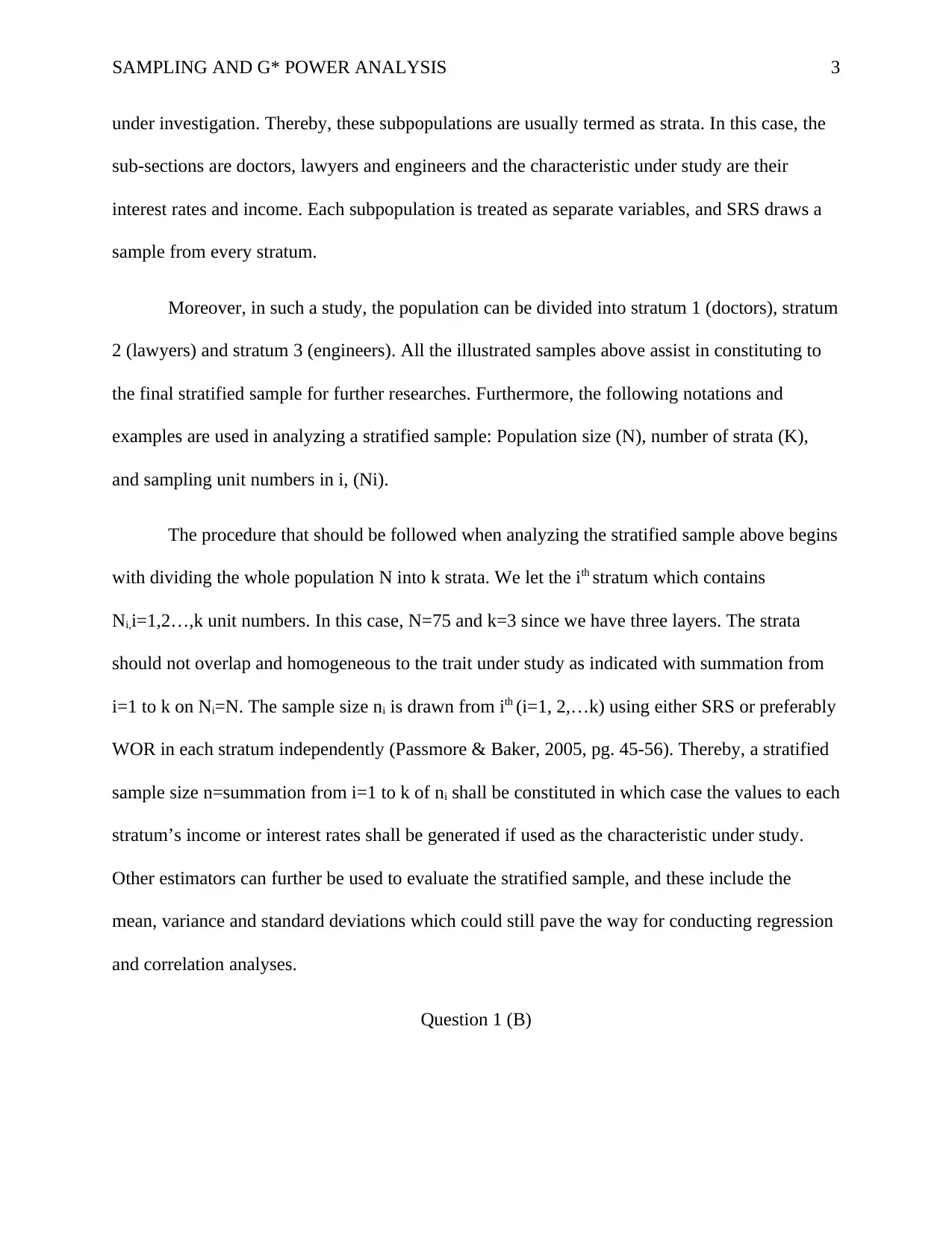
under investigation. Thereby, these subpopulations are usually termed as strata. In this case, the
sub-sections are doctors, lawyers and engineers and the characteristic under study are their
interest rates and income. Each subpopulation is treated as separate variables, and SRS draws a
sample from every stratum.
Moreover, in such a study, the population can be divided into stratum 1 (doctors), stratum
2 (lawyers) and stratum 3 (engineers). All the illustrated samples above assist in constituting to
the final stratified sample for further researches. Furthermore, the following notations and
examples are used in analyzing a stratified sample: Population size (N), number of strata (K),
and sampling unit numbers in i, (Ni).
The procedure that should be followed when analyzing the stratified sample above begins
with dividing the whole population N into k strata. We let the ith stratum which contains
Ni,i=1,2…,k unit numbers. In this case, N=75 and k=3 since we have three layers. The strata
should not overlap and homogeneous to the trait under study as indicated with summation from
i=1 to k on Ni=N. The sample size ni is drawn from ith (i=1, 2,…k) using either SRS or preferably
WOR in each stratum independently (Passmore & Baker, 2005, pg. 45-56). Thereby, a stratified
sample size n=summation from i=1 to k of ni shall be constituted in which case the values to each
stratum’s income or interest rates shall be generated if used as the characteristic under study.
Other estimators can further be used to evaluate the stratified sample, and these include the
mean, variance and standard deviations which could still pave the way for conducting regression
and correlation analyses.
Question 1 (B)
⊘ This is a preview!⊘
Do you want full access?
Subscribe today to unlock all pages.
Trusted by 1+ million students worldwide
SAMPLING AND G* POWER ANALYSIS 4
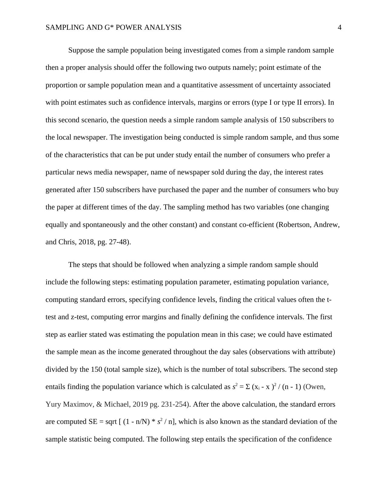
Suppose the sample population being investigated comes from a simple random sample
then a proper analysis should offer the following two outputs namely; point estimate of the
proportion or sample population mean and a quantitative assessment of uncertainty associated
with point estimates such as confidence intervals, margins or errors (type I or type II errors). In
this second scenario, the question needs a simple random sample analysis of 150 subscribers to
the local newspaper. The investigation being conducted is simple random sample, and thus some
of the characteristics that can be put under study entail the number of consumers who prefer a
particular news media newspaper, name of newspaper sold during the day, the interest rates
generated after 150 subscribers have purchased the paper and the number of consumers who buy
the paper at different times of the day. The sampling method has two variables (one changing
equally and spontaneously and the other constant) and constant co-efficient (Robertson, Andrew,
and Chris, 2018, pg. 27-48).
The steps that should be followed when analyzing a simple random sample should
include the following steps: estimating population parameter, estimating population variance,
computing standard errors, specifying confidence levels, finding the critical values often the t-
test and z-test, computing error margins and finally defining the confidence intervals. The first
step as earlier stated was estimating the population mean in this case; we could have estimated
the sample mean as the income generated throughout the day sales (observations with attribute)
divided by the 150 (total sample size), which is the number of total subscribers. The second step
entails finding the population variance which is calculated as s2 = Σ (xi - x )2 / (n - 1) (Owen,
Yury Maximov, & Michael, 2019 pg. 231-254). After the above calculation, the standard errors
are computed SE = sqrt [ (1 - n/N) * s2 / n], which is also known as the standard deviation of the
sample statistic being computed. The following step entails the specification of the confidence
Paraphrase This Document
Need a fresh take? Get an instant paraphrase of this document with our AI Paraphraser
SAMPLING AND G* POWER ANALYSIS 5
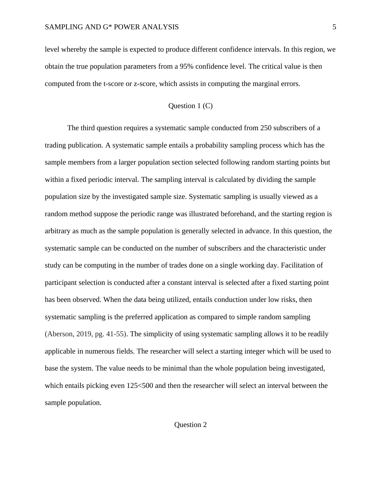
level whereby the sample is expected to produce different confidence intervals. In this region, we
obtain the true population parameters from a 95% confidence level. The critical value is then
computed from the t-score or z-score, which assists in computing the marginal errors.
Question 1 (C)
The third question requires a systematic sample conducted from 250 subscribers of a
trading publication. A systematic sample entails a probability sampling process which has the
sample members from a larger population section selected following random starting points but
within a fixed periodic interval. The sampling interval is calculated by dividing the sample
population size by the investigated sample size. Systematic sampling is usually viewed as a
random method suppose the periodic range was illustrated beforehand, and the starting region is
arbitrary as much as the sample population is generally selected in advance. In this question, the
systematic sample can be conducted on the number of subscribers and the characteristic under
study can be computing in the number of trades done on a single working day. Facilitation of
participant selection is conducted after a constant interval is selected after a fixed starting point
has been observed. When the data being utilized, entails conduction under low risks, then
systematic sampling is the preferred application as compared to simple random sampling
(Aberson, 2019, pg. 41-55). The simplicity of using systematic sampling allows it to be readily
applicable in numerous fields. The researcher will select a starting integer which will be used to
base the system. The value needs to be minimal than the whole population being investigated,
which entails picking even 125<500 and then the researcher will select an interval between the
sample population.
Question 2
SAMPLING AND G* POWER ANALYSIS 6
Part a
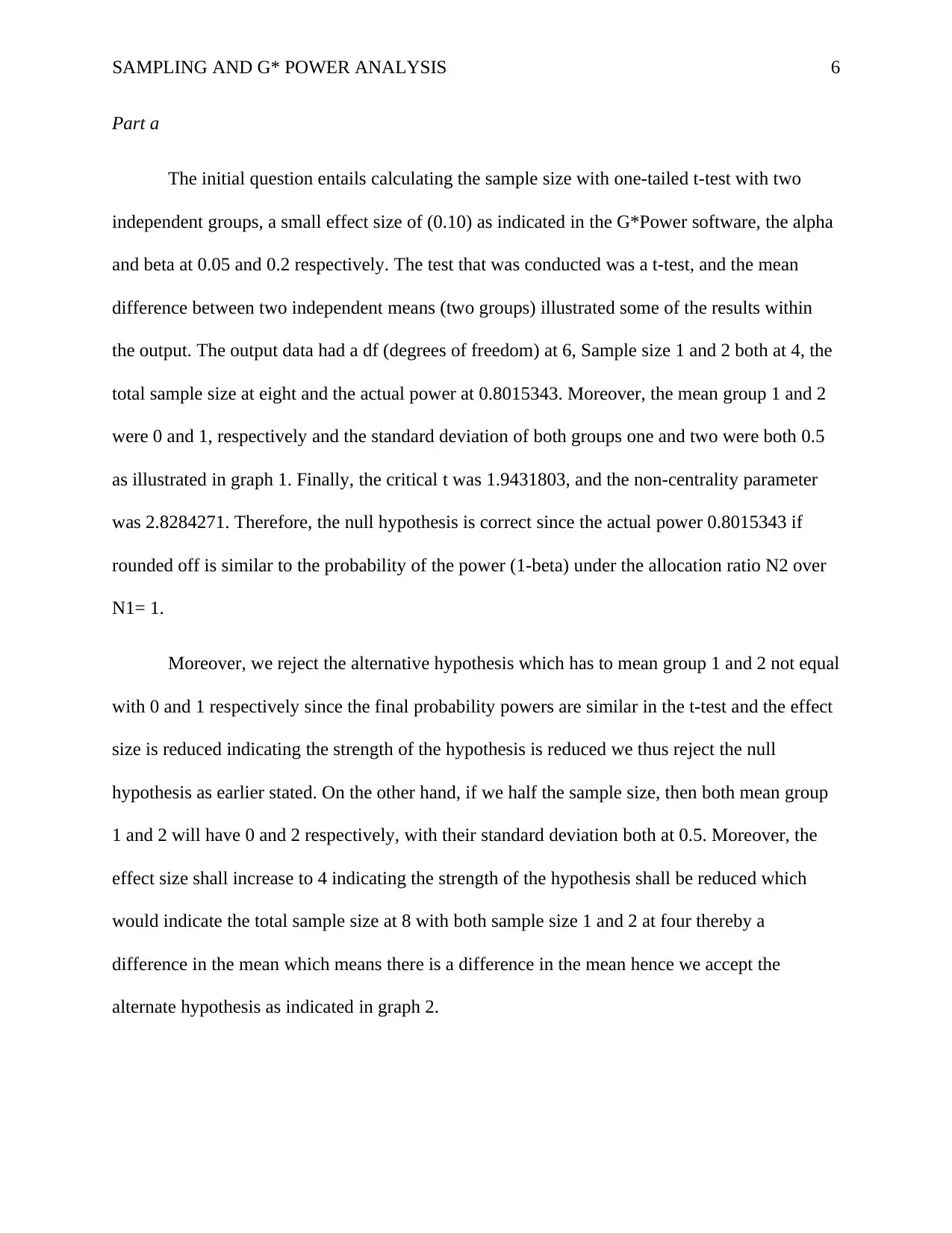
The initial question entails calculating the sample size with one-tailed t-test with two
independent groups, a small effect size of (0.10) as indicated in the G*Power software, the alpha
and beta at 0.05 and 0.2 respectively. The test that was conducted was a t-test, and the mean
difference between two independent means (two groups) illustrated some of the results within
the output. The output data had a df (degrees of freedom) at 6, Sample size 1 and 2 both at 4, the
total sample size at eight and the actual power at 0.8015343. Moreover, the mean group 1 and 2
were 0 and 1, respectively and the standard deviation of both groups one and two were both 0.5
as illustrated in graph 1. Finally, the critical t was 1.9431803, and the non-centrality parameter
was 2.8284271. Therefore, the null hypothesis is correct since the actual power 0.8015343 if
rounded off is similar to the probability of the power (1-beta) under the allocation ratio N2 over
N1= 1.
Moreover, we reject the alternative hypothesis which has to mean group 1 and 2 not equal
with 0 and 1 respectively since the final probability powers are similar in the t-test and the effect
size is reduced indicating the strength of the hypothesis is reduced we thus reject the null
hypothesis as earlier stated. On the other hand, if we half the sample size, then both mean group
1 and 2 will have 0 and 2 respectively, with their standard deviation both at 0.5. Moreover, the
effect size shall increase to 4 indicating the strength of the hypothesis shall be reduced which
would indicate the total sample size at 8 with both sample size 1 and 2 at four thereby a
difference in the mean which means there is a difference in the mean hence we accept the
alternate hypothesis as indicated in graph 2.
Part a
The initial question entails calculating the sample size with one-tailed t-test with two
independent groups, a small effect size of (0.10) as indicated in the G*Power software, the alpha
and beta at 0.05 and 0.2 respectively. The test that was conducted was a t-test, and the mean
difference between two independent means (two groups) illustrated some of the results within
the output. The output data had a df (degrees of freedom) at 6, Sample size 1 and 2 both at 4, the
total sample size at eight and the actual power at 0.8015343. Moreover, the mean group 1 and 2
were 0 and 1, respectively and the standard deviation of both groups one and two were both 0.5
as illustrated in graph 1. Finally, the critical t was 1.9431803, and the non-centrality parameter
was 2.8284271. Therefore, the null hypothesis is correct since the actual power 0.8015343 if
rounded off is similar to the probability of the power (1-beta) under the allocation ratio N2 over
N1= 1.
Moreover, we reject the alternative hypothesis which has to mean group 1 and 2 not equal
with 0 and 1 respectively since the final probability powers are similar in the t-test and the effect
size is reduced indicating the strength of the hypothesis is reduced we thus reject the null
hypothesis as earlier stated. On the other hand, if we half the sample size, then both mean group
1 and 2 will have 0 and 2 respectively, with their standard deviation both at 0.5. Moreover, the
effect size shall increase to 4 indicating the strength of the hypothesis shall be reduced which
would indicate the total sample size at 8 with both sample size 1 and 2 at four thereby a
difference in the mean which means there is a difference in the mean hence we accept the
alternate hypothesis as indicated in graph 2.
⊘ This is a preview!⊘
Do you want full access?
Subscribe today to unlock all pages.
Trusted by 1+ million students worldwide
SAMPLING AND G* POWER ANALYSIS 7
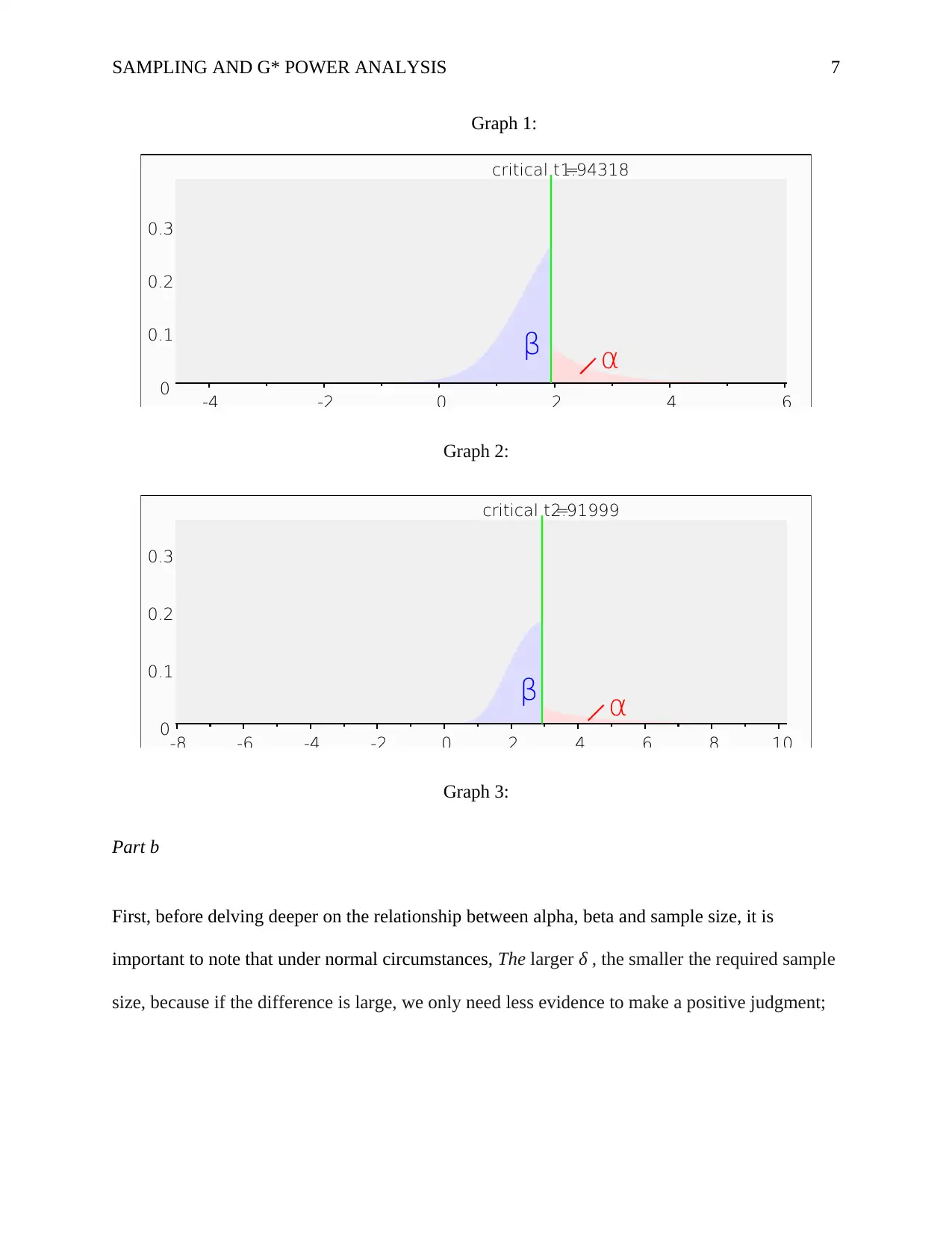
Graph 1:
0
0.1
0.2
0.3
-4 -2 0 2 4 6
critical t =1.94318
αβ
Graph 2:
0
0.1
0.2
0.3
-8 -6 -4 -2 0 2 4 6 8 10
critical t =2.91999
α
β
Graph 3:
Part b
First, before delving deeper on the relationship between alpha, beta and sample size, it is
important to note that under normal circumstances, The larger δ , the smaller the required sample
size, because if the difference is large, we only need less evidence to make a positive judgment;
Paraphrase This Document
Need a fresh take? Get an instant paraphrase of this document with our AI Paraphraser
SAMPLING AND G* POWER ANALYSIS 8
The larger σ, the larger the required sample size. It is easy to understand that more data is
needed to make the mean distribution thinner to ensure the power of the test. This is the central
limit theorem at work;
The larger α , the smaller the required sample size, because the area of rejection is
enlarged. The larger the power, the larger the sample size, because large power means that β is
small. According to the central limit theorem, under other conditions, the larger the sample size,
the thinner the distribution of the mean, making β smaller .
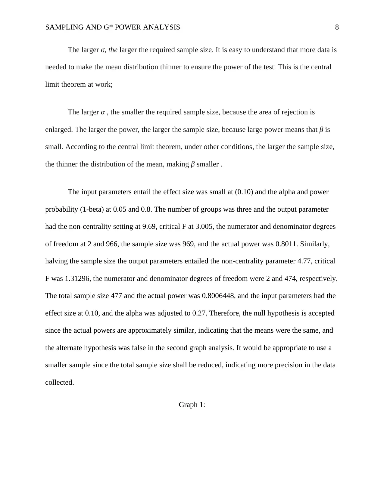
The input parameters entail the effect size was small at (0.10) and the alpha and power
probability (1-beta) at 0.05 and 0.8. The number of groups was three and the output parameter
had the non-centrality setting at 9.69, critical F at 3.005, the numerator and denominator degrees
of freedom at 2 and 966, the sample size was 969, and the actual power was 0.8011. Similarly,
halving the sample size the output parameters entailed the non-centrality parameter 4.77, critical
F was 1.31296, the numerator and denominator degrees of freedom were 2 and 474, respectively.
The total sample size 477 and the actual power was 0.8006448, and the input parameters had the
effect size at 0.10, and the alpha was adjusted to 0.27. Therefore, the null hypothesis is accepted
since the actual powers are approximately similar, indicating that the means were the same, and
the alternate hypothesis was false in the second graph analysis. It would be appropriate to use a
smaller sample since the total sample size shall be reduced, indicating more precision in the data
collected.
Graph 1:
The larger σ, the larger the required sample size. It is easy to understand that more data is
needed to make the mean distribution thinner to ensure the power of the test. This is the central
limit theorem at work;
The larger α , the smaller the required sample size, because the area of rejection is
enlarged. The larger the power, the larger the sample size, because large power means that β is
small. According to the central limit theorem, under other conditions, the larger the sample size,
the thinner the distribution of the mean, making β smaller .
The input parameters entail the effect size was small at (0.10) and the alpha and power
probability (1-beta) at 0.05 and 0.8. The number of groups was three and the output parameter
had the non-centrality setting at 9.69, critical F at 3.005, the numerator and denominator degrees
of freedom at 2 and 966, the sample size was 969, and the actual power was 0.8011. Similarly,
halving the sample size the output parameters entailed the non-centrality parameter 4.77, critical
F was 1.31296, the numerator and denominator degrees of freedom were 2 and 474, respectively.
The total sample size 477 and the actual power was 0.8006448, and the input parameters had the
effect size at 0.10, and the alpha was adjusted to 0.27. Therefore, the null hypothesis is accepted
since the actual powers are approximately similar, indicating that the means were the same, and
the alternate hypothesis was false in the second graph analysis. It would be appropriate to use a
smaller sample since the total sample size shall be reduced, indicating more precision in the data
collected.
Graph 1:
SAMPLING AND G* POWER ANALYSIS 9
0
0.2
0.4
0.6
0.8
1
0 2 4 6 8 10 12
critical F =3.00504
αβ
Graph 2:
0
0.2
0.4
0.6
0.8
1
0 1 2 3 4 5 6 7
critical F =1.31296
αβ
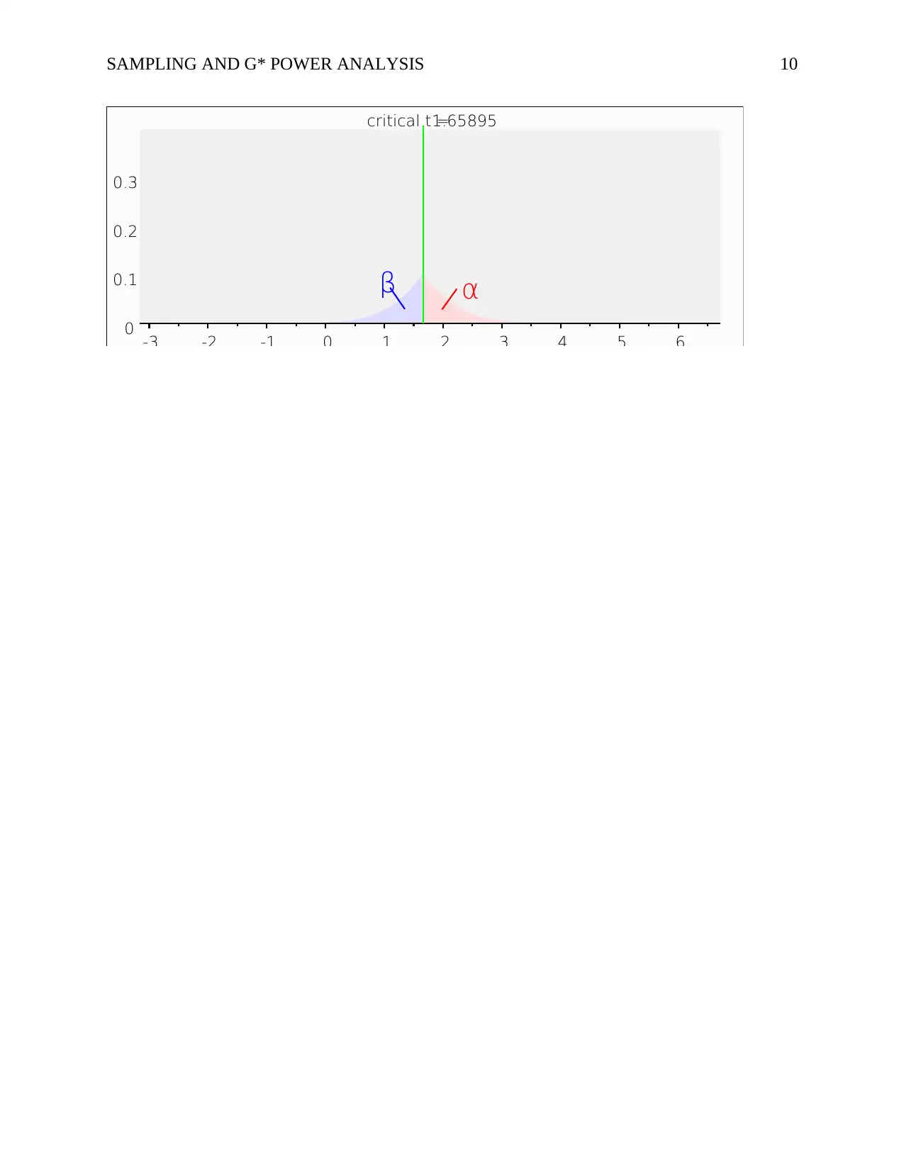
Question 3
The sampling method that would be appropriate for my study would be t-test one-tailed,
and the specific population size would be 111. The degrees of freedom would be 109; the actual
power would be 0.9503016 and the non-centrality parameter 3.3133098 within the output
parameters. On the other hand, the input parameters would have the effect size at medium (0.3),
the alpha probability would be 0.05, and the power probability (1-beta) would be 0.95. The
statistical test could be collected based on the point biserial model (correlation).
0
0.2
0.4
0.6
0.8
1
0 2 4 6 8 10 12
critical F =3.00504
αβ
Graph 2:
0
0.2
0.4
0.6
0.8
1
0 1 2 3 4 5 6 7
critical F =1.31296
αβ
Question 3
The sampling method that would be appropriate for my study would be t-test one-tailed,
and the specific population size would be 111. The degrees of freedom would be 109; the actual
power would be 0.9503016 and the non-centrality parameter 3.3133098 within the output
parameters. On the other hand, the input parameters would have the effect size at medium (0.3),
the alpha probability would be 0.05, and the power probability (1-beta) would be 0.95. The
statistical test could be collected based on the point biserial model (correlation).
⊘ This is a preview!⊘
Do you want full access?
Subscribe today to unlock all pages.
Trusted by 1+ million students worldwide
SAMPLING AND G* POWER ANALYSIS 10
0
0.1
0.2
0.3
-3 -2 -1 0 1 2 3 4 5 6
critical t =1.65895
αβ
0
0.1
0.2
0.3
-3 -2 -1 0 1 2 3 4 5 6
critical t =1.65895
αβ
Paraphrase This Document
Need a fresh take? Get an instant paraphrase of this document with our AI Paraphraser
SAMPLING AND G* POWER ANALYSIS 11
References
Aberson, C. L. (2019). Applied power analysis for the behavioural sciences. Routledge.
Green, P., and Catriona J. M. (2016). SIMR: An R package for power analysis of generalized
linear mixed models by simulation. Methods in Ecology and Evolution 7 (4): 493-498.
Mumby, P. J. (2002). Statistical power of non-parametric tests: A quick guide for designing
sampling strategies. Marine pollution bulletin, 44(1): 85-87.
Owen, A. B., Yury M., and Michael C. (2019). Importance sampling the union of rare events
with an application to power systems analysis. Electronic Journal of Statistics 13 (1):
231-254.
Passmore, D. L., & Baker, R. M. (2005). Sampling strategies and power analysis. Research in
organizations: Foundations and methods of inquiry 6(1): 45-56.
Robertson, A., and Chris G. S. (2018). Research sampling: a pragmatic approach." Advanced
Research Methods for Applied Psychology. Routledge.
1 out of 11


Your All-in-One AI-Powered Toolkit for Academic Success.
+13062052269
info@desklib.com
Available 24*7 on WhatsApp / Email
![[object Object]](/_next/static/media/star-bottom.7253800d.svg)
Unlock your academic potential
Copyright © 2020–2026 A2Z Services. All Rights Reserved. Developed and managed by ZUCOL.