BUS5CA Assignment 1: Social Media Analysis Using SAS Text Miner
VerifiedAdded on 2022/12/27
|8
|1446
|313
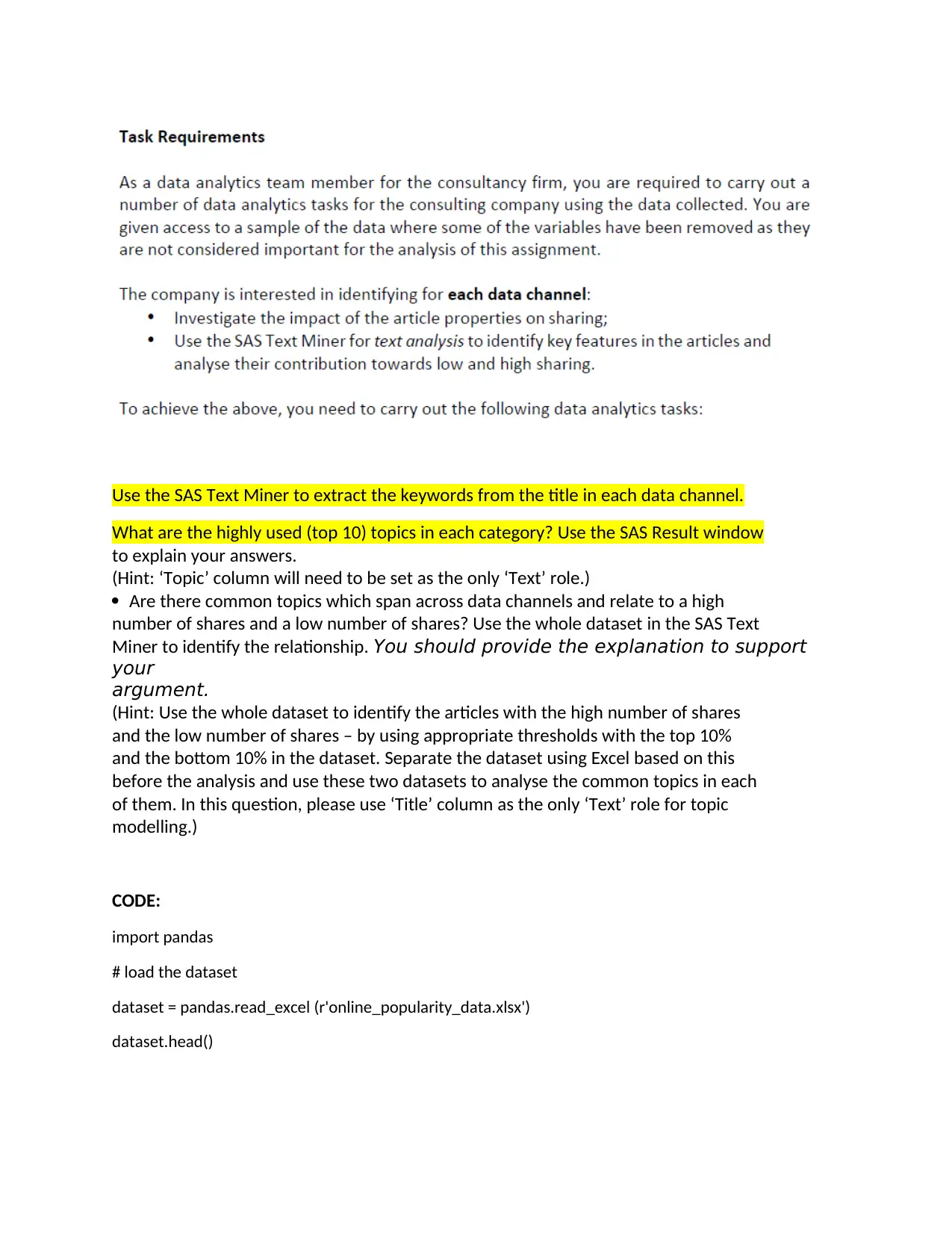
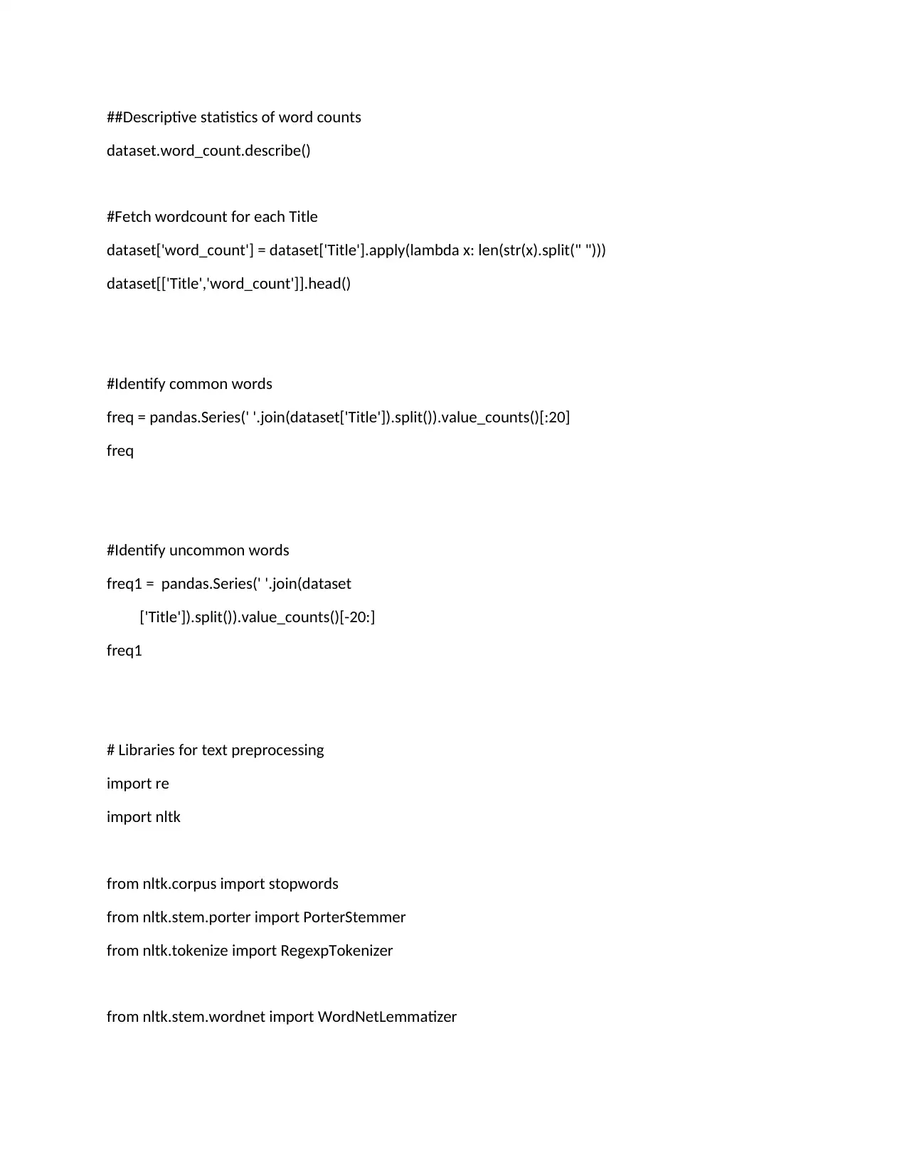
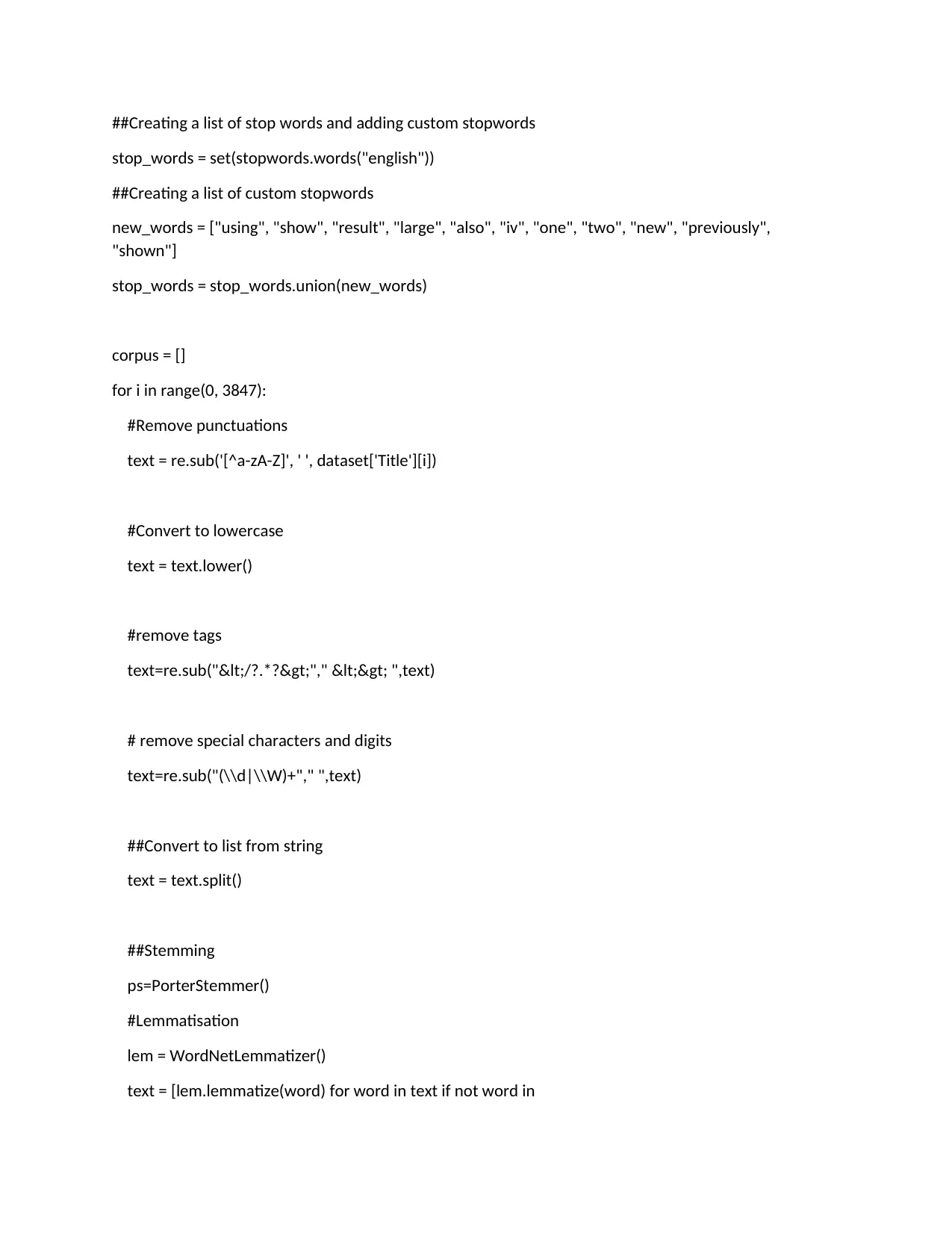
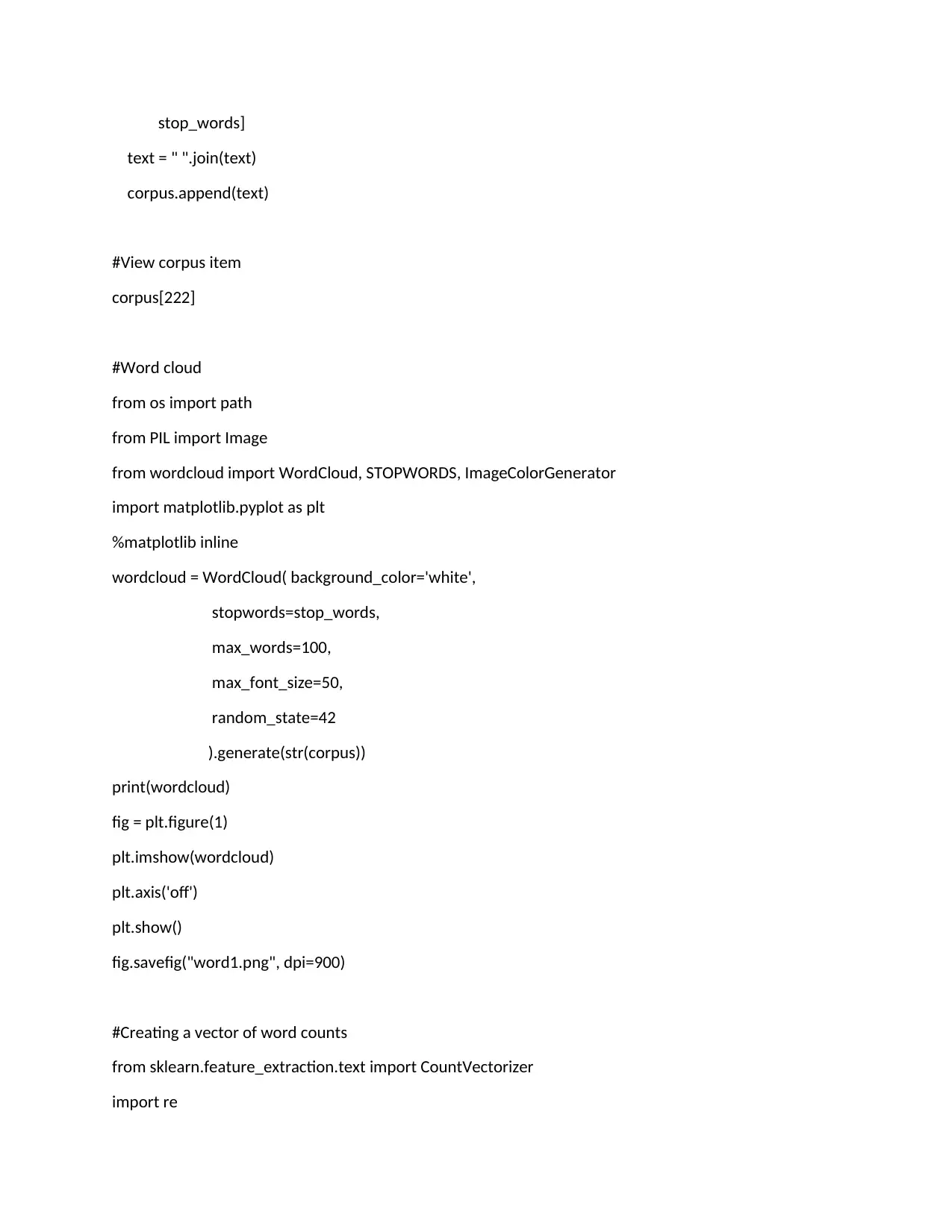
Practical Assignment
AI Summary
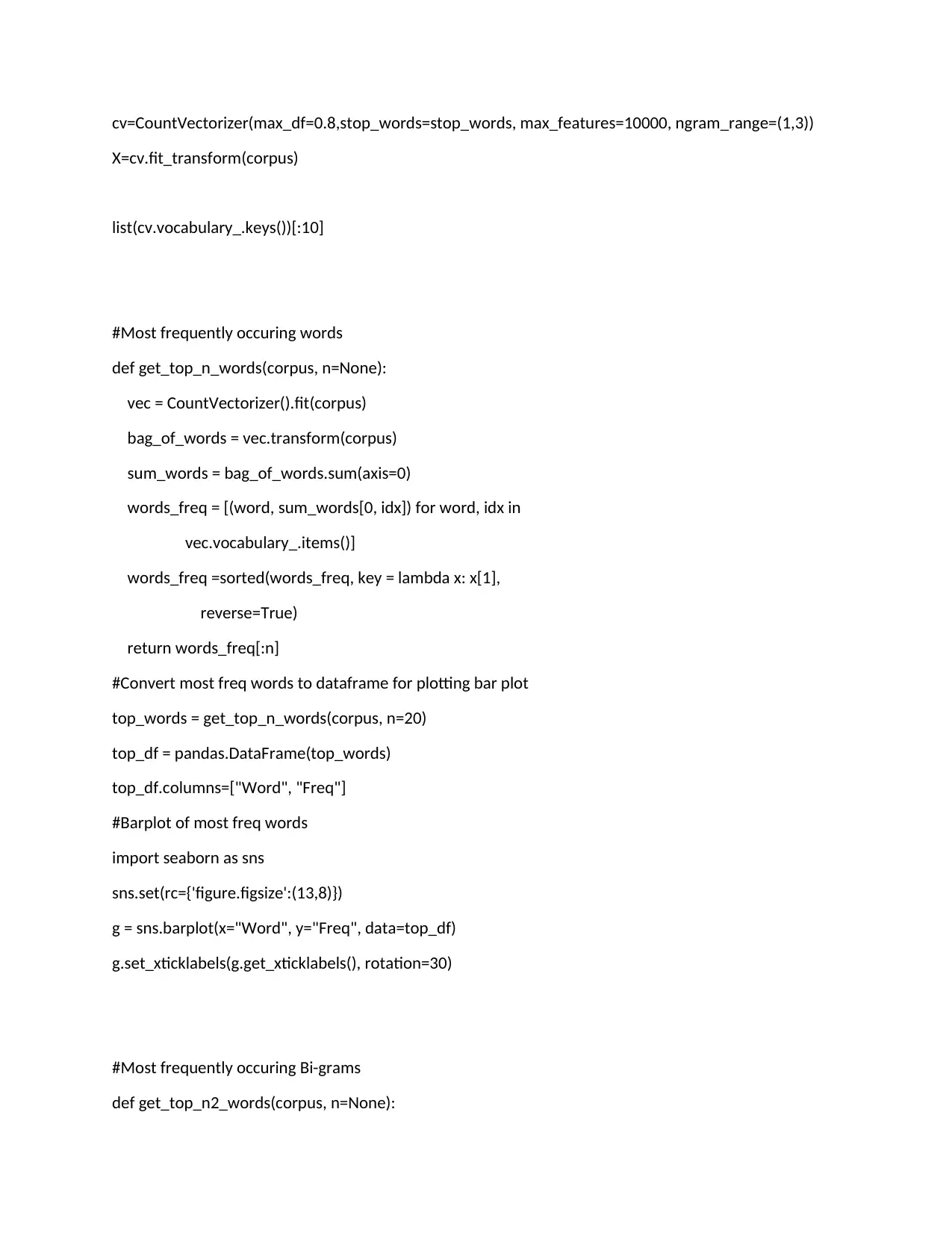
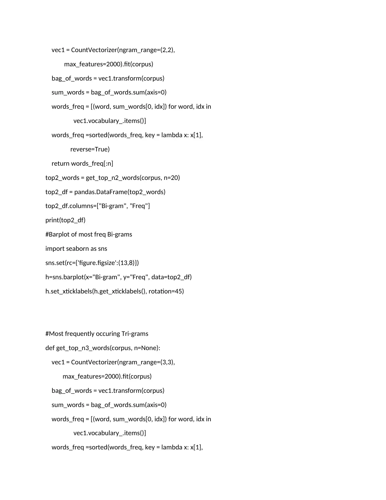
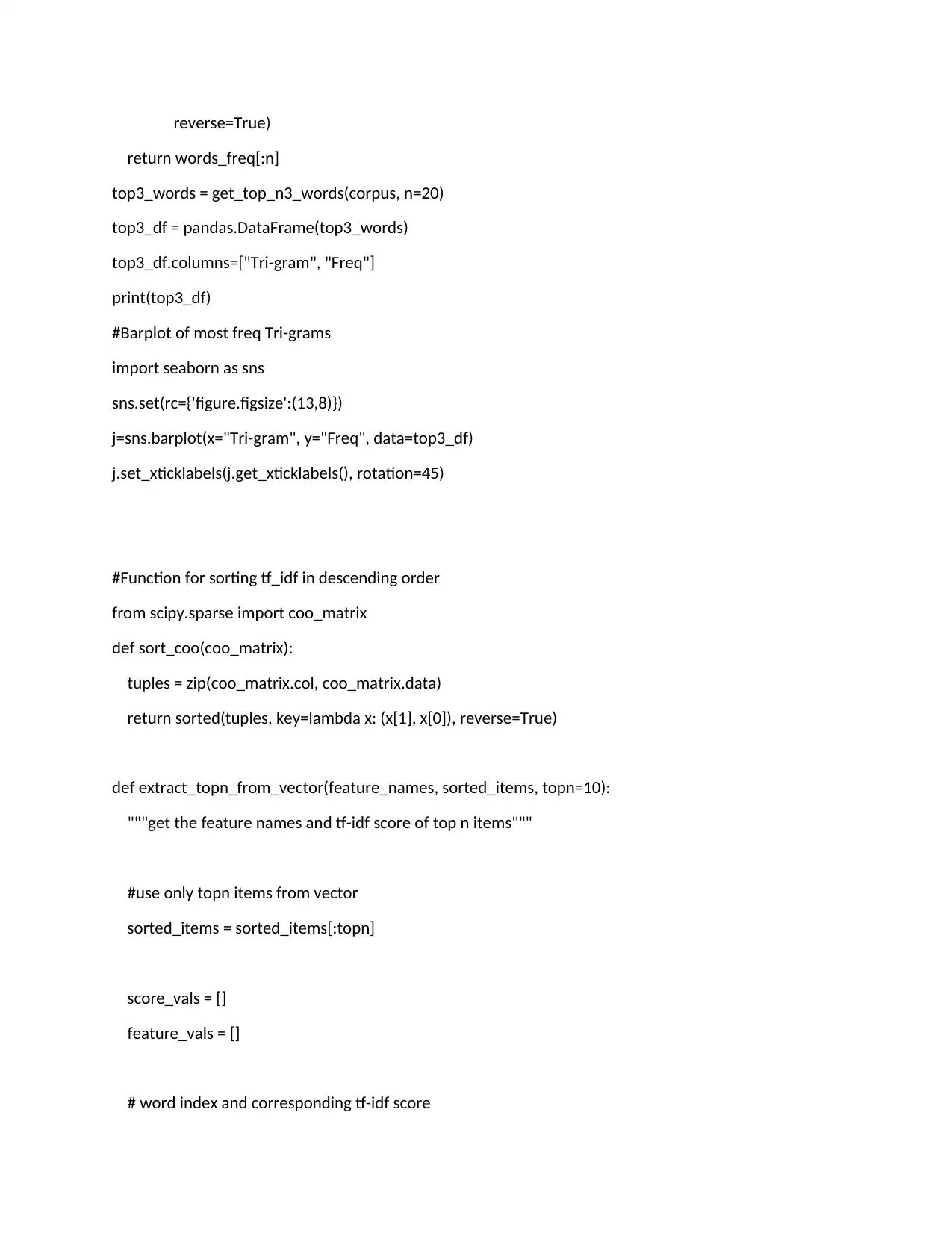
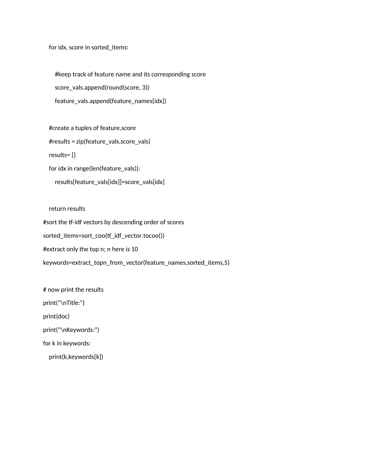
This assignment, completed for the BUS5CA Customer Analytics and Social Media course, utilizes SAS Text Miner to analyze social media data and understand customer preferences. The task involves extracting keywords from article titles across different data channels and identifying the top...

Use the SAS Text Miner to extract the keywords from the title in each data channel.
What are the highly used (top 10) topics in each category? Use the SAS Result window
to explain your answers.
(Hint: ‘Topic’ column will need to be set as the only ‘Text’ role.)
Are there common topics which span across data channels and relate to a high
number of shares and a low number of shares? Use the whole dataset in the SAS Text
Miner to identify the relationship. You should provide the explanation to support
your
argument.
(Hint: Use the whole dataset to identify the articles with the high number of shares
and the low number of shares – by using appropriate thresholds with the top 10%
and the bottom 10% in the dataset. Separate the dataset using Excel based on this
before the analysis and use these two datasets to analyse the common topics in each
of them. In this question, please use ‘Title’ column as the only ‘Text’ role for topic
modelling.)
CODE:
import pandas
# load the dataset
dataset = pandas.read_excel (r'online_popularity_data.xlsx')
dataset.head()
Paraphrase This Document
Need a fresh take? Get an instant paraphrase of this document with our AI Paraphraser

##Descriptive statistics of word counts
dataset.word_count.describe()
#Fetch wordcount for each Title
dataset['word_count'] = dataset['Title'].apply(lambda x: len(str(x).split(" ")))
dataset[['Title','word_count']].head()
#Identify common words
freq = pandas.Series(' '.join(dataset['Title']).split()).value_counts()[:20]
freq
#Identify uncommon words
freq1 = pandas.Series(' '.join(dataset
['Title']).split()).value_counts()[-20:]
freq1
# Libraries for text preprocessing
import re
import nltk
from nltk.corpus import stopwords
from nltk.stem.porter import PorterStemmer
from nltk.tokenize import RegexpTokenizer
from nltk.stem.wordnet import WordNetLemmatizer

##Creating a list of stop words and adding custom stopwords
stop_words = set(stopwords.words("english"))
##Creating a list of custom stopwords
new_words = ["using", "show", "result", "large", "also", "iv", "one", "two", "new", "previously",
"shown"]
stop_words = stop_words.union(new_words)
corpus = []
for i in range(0, 3847):
#Remove punctuations
text = re.sub('[^a-zA-Z]', ' ', dataset['Title'][i])
#Convert to lowercase
text = text.lower()
#remove tags
text=re.sub("</?.*?>"," <> ",text)
# remove special characters and digits
text=re.sub("(\\d|\\W)+"," ",text)
##Convert to list from string
text = text.split()
##Stemming
ps=PorterStemmer()
#Lemmatisation
lem = WordNetLemmatizer()
text = [lem.lemmatize(word) for word in text if not word in
⊘ This is a preview!⊘
Do you want full access?
Subscribe today to unlock all pages.

Trusted by 1+ million students worldwide

stop_words]
text = " ".join(text)
corpus.append(text)
#View corpus item
corpus[222]
#Word cloud
from os import path
from PIL import Image
from wordcloud import WordCloud, STOPWORDS, ImageColorGenerator
import matplotlib.pyplot as plt
%matplotlib inline
wordcloud = WordCloud( background_color='white',
stopwords=stop_words,
max_words=100,
max_font_size=50,
random_state=42
).generate(str(corpus))
print(wordcloud)
fig = plt.figure(1)
plt.imshow(wordcloud)
plt.axis('off')
plt.show()
fig.savefig("word1.png", dpi=900)
#Creating a vector of word counts
from sklearn.feature_extraction.text import CountVectorizer
import re
Paraphrase This Document
Need a fresh take? Get an instant paraphrase of this document with our AI Paraphraser

cv=CountVectorizer(max_df=0.8,stop_words=stop_words, max_features=10000, ngram_range=(1,3))
X=cv.fit_transform(corpus)
list(cv.vocabulary_.keys())[:10]
#Most frequently occuring words
def get_top_n_words(corpus, n=None):
vec = CountVectorizer().fit(corpus)
bag_of_words = vec.transform(corpus)
sum_words = bag_of_words.sum(axis=0)
words_freq = [(word, sum_words[0, idx]) for word, idx in
vec.vocabulary_.items()]
words_freq =sorted(words_freq, key = lambda x: x[1],
reverse=True)
return words_freq[:n]
#Convert most freq words to dataframe for plotting bar plot
top_words = get_top_n_words(corpus, n=20)
top_df = pandas.DataFrame(top_words)
top_df.columns=["Word", "Freq"]
#Barplot of most freq words
import seaborn as sns
sns.set(rc={'figure.figsize':(13,8)})
g = sns.barplot(x="Word", y="Freq", data=top_df)
g.set_xticklabels(g.get_xticklabels(), rotation=30)
#Most frequently occuring Bi-grams
def get_top_n2_words(corpus, n=None):

vec1 = CountVectorizer(ngram_range=(2,2),
max_features=2000).fit(corpus)
bag_of_words = vec1.transform(corpus)
sum_words = bag_of_words.sum(axis=0)
words_freq = [(word, sum_words[0, idx]) for word, idx in
vec1.vocabulary_.items()]
words_freq =sorted(words_freq, key = lambda x: x[1],
reverse=True)
return words_freq[:n]
top2_words = get_top_n2_words(corpus, n=20)
top2_df = pandas.DataFrame(top2_words)
top2_df.columns=["Bi-gram", "Freq"]
print(top2_df)
#Barplot of most freq Bi-grams
import seaborn as sns
sns.set(rc={'figure.figsize':(13,8)})
h=sns.barplot(x="Bi-gram", y="Freq", data=top2_df)
h.set_xticklabels(h.get_xticklabels(), rotation=45)
#Most frequently occuring Tri-grams
def get_top_n3_words(corpus, n=None):
vec1 = CountVectorizer(ngram_range=(3,3),
max_features=2000).fit(corpus)
bag_of_words = vec1.transform(corpus)
sum_words = bag_of_words.sum(axis=0)
words_freq = [(word, sum_words[0, idx]) for word, idx in
vec1.vocabulary_.items()]
words_freq =sorted(words_freq, key = lambda x: x[1],
max_features=2000).fit(corpus)
bag_of_words = vec1.transform(corpus)
sum_words = bag_of_words.sum(axis=0)
words_freq = [(word, sum_words[0, idx]) for word, idx in
vec1.vocabulary_.items()]
words_freq =sorted(words_freq, key = lambda x: x[1],
reverse=True)
return words_freq[:n]
top2_words = get_top_n2_words(corpus, n=20)
top2_df = pandas.DataFrame(top2_words)
top2_df.columns=["Bi-gram", "Freq"]
print(top2_df)
#Barplot of most freq Bi-grams
import seaborn as sns
sns.set(rc={'figure.figsize':(13,8)})
h=sns.barplot(x="Bi-gram", y="Freq", data=top2_df)
h.set_xticklabels(h.get_xticklabels(), rotation=45)
#Most frequently occuring Tri-grams
def get_top_n3_words(corpus, n=None):
vec1 = CountVectorizer(ngram_range=(3,3),
max_features=2000).fit(corpus)
bag_of_words = vec1.transform(corpus)
sum_words = bag_of_words.sum(axis=0)
words_freq = [(word, sum_words[0, idx]) for word, idx in
vec1.vocabulary_.items()]
words_freq =sorted(words_freq, key = lambda x: x[1],
⊘ This is a preview!⊘
Do you want full access?
Subscribe today to unlock all pages.

Trusted by 1+ million students worldwide

reverse=True)
return words_freq[:n]
top3_words = get_top_n3_words(corpus, n=20)
top3_df = pandas.DataFrame(top3_words)
top3_df.columns=["Tri-gram", "Freq"]
print(top3_df)
#Barplot of most freq Tri-grams
import seaborn as sns
sns.set(rc={'figure.figsize':(13,8)})
j=sns.barplot(x="Tri-gram", y="Freq", data=top3_df)
j.set_xticklabels(j.get_xticklabels(), rotation=45)
#Function for sorting tf_idf in descending order
from scipy.sparse import coo_matrix
def sort_coo(coo_matrix):
tuples = zip(coo_matrix.col, coo_matrix.data)
return sorted(tuples, key=lambda x: (x[1], x[0]), reverse=True)
def extract_topn_from_vector(feature_names, sorted_items, topn=10):
"""get the feature names and tf-idf score of top n items"""
#use only topn items from vector
sorted_items = sorted_items[:topn]
score_vals = []
feature_vals = []
# word index and corresponding tf-idf score
Paraphrase This Document
Need a fresh take? Get an instant paraphrase of this document with our AI Paraphraser

for idx, score in sorted_items:
#keep track of feature name and its corresponding score
score_vals.append(round(score, 3))
feature_vals.append(feature_names[idx])
#create a tuples of feature,score
#results = zip(feature_vals,score_vals)
results= {}
for idx in range(len(feature_vals)):
results[feature_vals[idx]]=score_vals[idx]
return results
#sort the tf-idf vectors by descending order of scores
sorted_items=sort_coo(tf_idf_vector.tocoo())
#extract only the top n; n here is 10
keywords=extract_topn_from_vector(feature_names,sorted_items,5)
# now print the results
print("\nTitle:")
print(doc)
print("\nKeywords:")
for k in keywords:
print(k,keywords[k])
1 out of 8

Your All-in-One AI-Powered Toolkit for Academic Success.
+13062052269
info@desklib.com
Available 24*7 on WhatsApp / Email
Unlock your academic potential
© 2024 | Zucol Services PVT LTD | All rights reserved.