SC504: Analyzing Income Disparities with NCDS - Height, Sex & Class
VerifiedAdded on 2023/06/03
|16
|2864
|178
Report
AI Summary
This report investigates the factors influencing net income using data from the National Child Development Study (NCDS). Three regression models were employed to analyze the relationship between net income and variables such as height, sex, reading ability, and parental social class. The findings suggest a significant relationship between height, sex, reading ability, and net earnings, while no significant relationship was found between parental social class and net income. The analysis reveals that taller individuals and those with better reading abilities tend to earn more, and that gender plays a role in income disparities. The report provides a detailed analysis of these relationships, supported by regression diagnostics and hypothesis testing, offering insights into the determinants of income based on the NCDS dataset.
1
Quantitative Analysis
Abstract
An indication of one’s effort in work has been for long time been thought to be reflected in the
individual’s net income. In this paper, we explore several factors such as height, sex, ability to
read (education) as well as parental social class and how they are related to net income. After
using 3 regression models to fit the independent variable net income against other response
variable in the dataset we conclude that there is a relationship between height, sex and ability to
read and one’s net earnings while there is no relationship between parental social class and net
income.
Key words
Elaboration framework, Regression, socioeconomic status
Paraphrase This Document
Need a fresh take? Get an instant paraphrase of this document with our AI Paraphraser
2
Quantitative Analysis
1. Introduction
1.1 Background information
Since the age of industrialization and even well before that, there have been curiosity to
realize what characterizes the pay that a given employee gets. In a salary survey conducted by
Zabel (2015) to determine what kind of factors influence salaries, several factors such as level of
education, overtime working and skills are proposed. For instance, in the study outcome, a job
whose position is hardest to fill attracted higher pay compared to that whose market is saturated.
Another research conducted in the mid-1990s indicated that there was a general salary gap
between male and females (Aizer, 2010), this therefore, suggests that sex is another factor that is
likely to cause salary difference.
1.2 Purpose of study
The purpose of this study is to:
i. Determine whether tall people earn more than others
ii. Determine if one’s ability to read, sex, parental social class as well as height do influence
earnings of an individual
1.3 Problem statement
From the purpose of the research, the problem is therefore to examine the factors that affect
earnings, i.e. “Is there a relationship between salary and factors such as height, sex, ability to
read and social class?”
3
Quantitative Analysis
1.4 Research questions
At the end of our research, we need to answer the following three questions:
Does height influence an individual’s net earnings?
Is there a relationship between reading ability, sex, and parental social class?
Is there a relationship between reading ability, sex, parental social class, and height?
⊘ This is a preview!⊘
Do you want full access?
Subscribe today to unlock all pages.
Trusted by 1+ million students worldwide

4
Quantitative Analysis
2. Literature Review
2.1 Social class stratification
In about the middle period of industrialization, around 1851 in Britain, there begun an
exercise to classify the British population according to occupation and industry (Rose, 1995). In
general, the population was stratified into the following classes:
i. Professional occupations
ii. Managerial and Technical occupations
iii. Skilled occupations i.e. “Non-manual” and “Manual”
iv. Partly skilled occupations
v. Unskilled occupations
Therefore, classification according to social classes occurred among working persons and has
become the basis of societal class stratification.
2.2 Parental social class
Erola and Lehti (2016) in their social paper on social stratification and mobility argue that,
“…despite relatively high degree of equality of opportunity in most of the developed countries,
family background still influences inheritance of social classes.” As such, the socioeconomic
status tend to influence each other, i.e. education, class and income (Crowford and Erve 2015)
2.3 Sex (Gender and earnings)
In a research on gender and income disparities, Ruel and Hauser (2013) note that there is an
identifiable income gap between male and female. More especially, there is a large wealth
Paraphrase This Document
Need a fresh take? Get an instant paraphrase of this document with our AI Paraphraser
5
Quantitative Analysis
accumulation gap between married men and married women, such differences are attributed to
investment strategies and selection effects. Additionally, households that have a single parent
accumulate less wealth compared to those with two parent, i.e. the married (Schmidt and Sevak,
2005).
2.4 Height
Past studies indicate that there is little preference for short persons more so short men,
according to a study by Gregory in the 1960s. Pinsker (2015) argues that, “an extra inch
correlates to an estimated $800 in increased annual earnings.” These differences are attributed to
the fallacy that tall persons especially men (gender disparity as well) are often stronger and get
picked to do most task which are idealized to require strength. In the post by the Atlantic, it is
noted that among men those whose height is between 5’4’’ and 5’6’’ have the steepest earning
differences.
2.5 Lazarsfeldian theoretical framework
2.1.1 Hypothesis
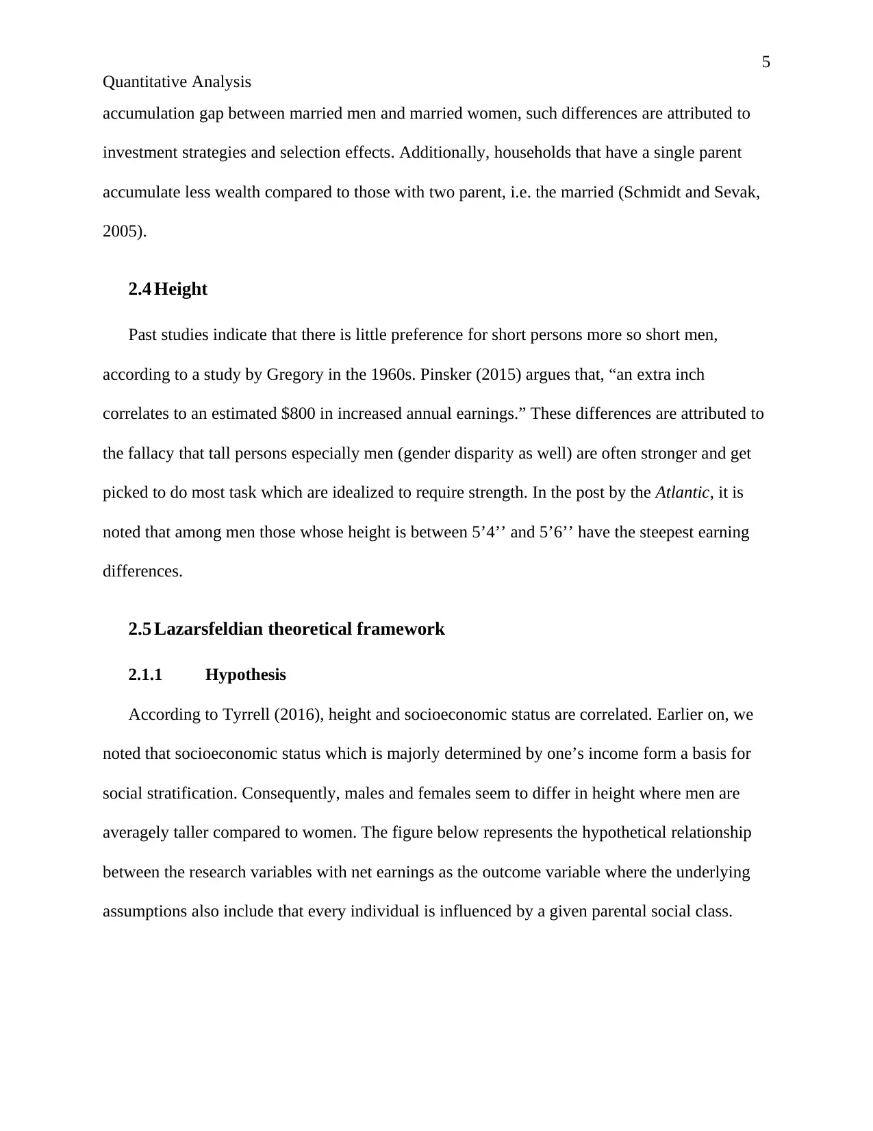
According to Tyrrell (2016), height and socioeconomic status are correlated. Earlier on, we
noted that socioeconomic status which is majorly determined by one’s income form a basis for
social stratification. Consequently, males and females seem to differ in height where men are
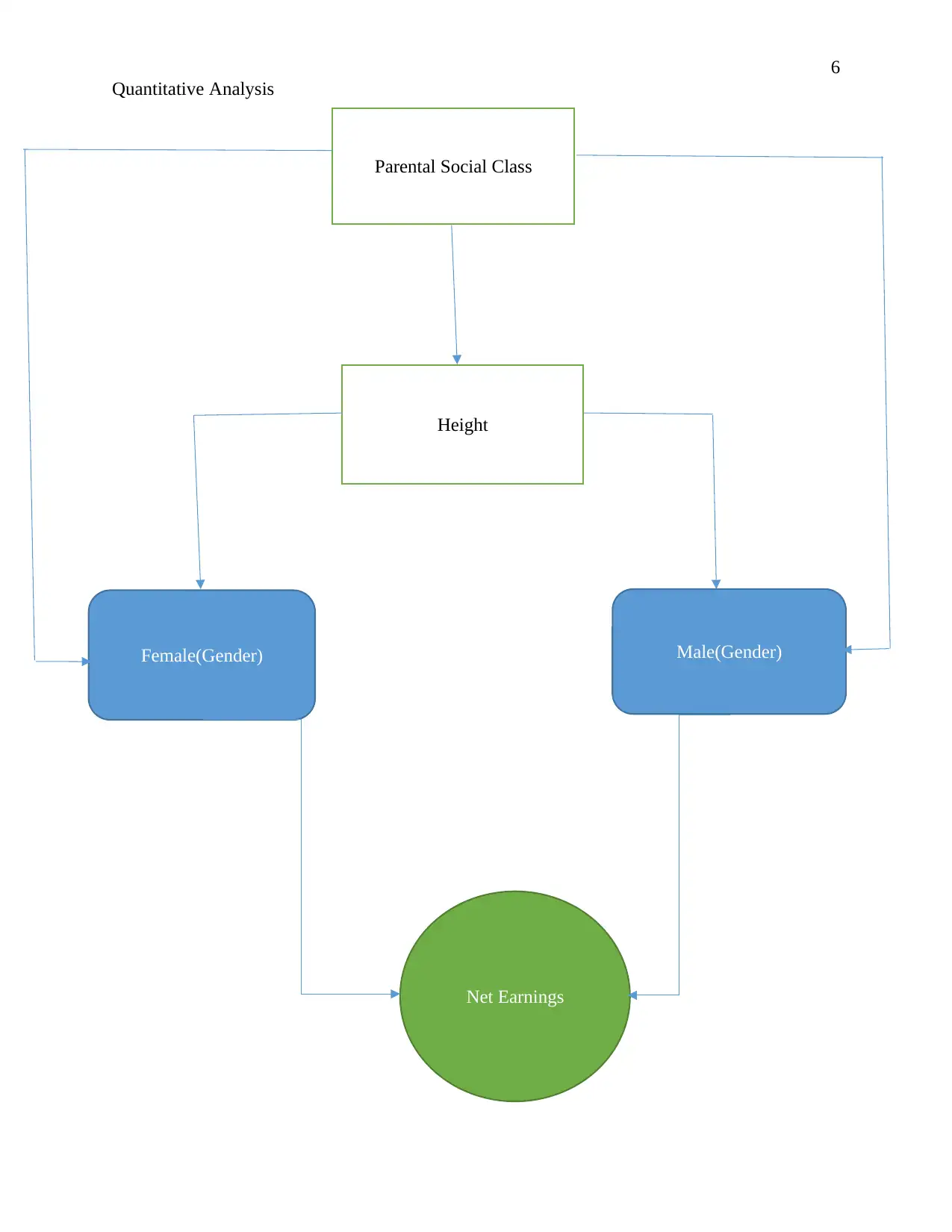
averagely taller compared to women. The figure below represents the hypothetical relationship
between the research variables with net earnings as the outcome variable where the underlying
assumptions also include that every individual is influenced by a given parental social class.
Quantitative Analysis
accumulation gap between married men and married women, such differences are attributed to
investment strategies and selection effects. Additionally, households that have a single parent
accumulate less wealth compared to those with two parent, i.e. the married (Schmidt and Sevak,
2005).
2.4 Height
Past studies indicate that there is little preference for short persons more so short men,
according to a study by Gregory in the 1960s. Pinsker (2015) argues that, “an extra inch
correlates to an estimated $800 in increased annual earnings.” These differences are attributed to
the fallacy that tall persons especially men (gender disparity as well) are often stronger and get
picked to do most task which are idealized to require strength. In the post by the Atlantic, it is
noted that among men those whose height is between 5’4’’ and 5’6’’ have the steepest earning
differences.
2.5 Lazarsfeldian theoretical framework
2.1.1 Hypothesis
According to Tyrrell (2016), height and socioeconomic status are correlated. Earlier on, we
noted that socioeconomic status which is majorly determined by one’s income form a basis for
social stratification. Consequently, males and females seem to differ in height where men are
averagely taller compared to women. The figure below represents the hypothetical relationship
between the research variables with net earnings as the outcome variable where the underlying
assumptions also include that every individual is influenced by a given parental social class.
6
Quantitative Analysis
Parental Social Class
Height
Female(Gender) Male(Gender)
Net Earnings
Quantitative Analysis
Parental Social Class
Height
Female(Gender) Male(Gender)
Net Earnings
⊘ This is a preview!⊘
Do you want full access?
Subscribe today to unlock all pages.
Trusted by 1+ million students worldwide
7
Quantitative Analysis
3. Methodology
3.1 Data
Data for this research is obtained from UK data service. It contains 7 variables i.e.: Gender (Sex),
Net earnings, Height, Parental social class, Ability to read, intmth11, and Female
3.1.1 Data management
During data cleaning and management, the sex variable is renamed to gender while the
female variable is dropped altogether due to its redundant nature, i.e. the female and gender
variables serve the same purpose such that they both indicate whether a respondent is male or
female. Another variable that is not useful for our data analysis is the intmth11 which is dropped
from the dataset. In addition, the netearn23 is renamed to Net earnings, height23 is renamed to
Height and read11 to Read. The gender variable is coded such that, 1-Male, 2-Female. The
parental social classes are coded from 1:6 with 1 being the highest social class while 6 is the
lowest and is renamed to Class from class16.
3.2 Regression
Our original interest is to determine the relationship between net earnings and other predictor
variables. Given the three research questions, we fit three regression models with net earnings
being the response variables and in the 1st equation height being the only predictor variable. In
the 2nd regression equation, reading ability, sex, and parental social class are the predictor
variables while in the last equation, all the variables excluding net earnings which is the predictor
variable in thee dataset are independent variables as in the equations below:
i. Yi=β0+β1X1+ £I, where: β0 is the regression coefficient
Paraphrase This Document
Need a fresh take? Get an instant paraphrase of this document with our AI Paraphraser
8
Quantitative Analysis
β1 is the coefficient of predictor variable X1 height
£i is the random error term
Yi is the response variable net earnings
ii. Yi=β0+β1X1+ β2X2+ β3X3+£I, where: β0 is the regression coefficient
β1 is the coefficient of predictor variable X1 reading ability
β2 is the coefficient of predictor variable X2 sex
β3 is the coefficient of predictor variable X3 Parental social class
£i is the random error term
Yi is the response variable net earnings
iii. Yi=β0+β1X1+ β2X2+ β3X3+ β4X4+£I, where: β0 is the regression coefficient
β1 is the coefficient of predictor variable X1 reading ability
β2 is the coefficient of predictor variable X2 sex
β3 is the coefficient of predictor variable X3 Parental social class
β4 is the coefficient of predictor variable X4 height
£i is the random error term
Yi is the response variable net earnings
3.3 Hypotheses
To help in answering the research questions, three sets of hypotheses are formulated:
9
Quantitative Analysis
3.3.1 Hypothesis 1
Null hypothesis
Taller persons earn just like any other persons
Alternative hypothesis
Taller persons earn more than other persons, i.e. there is a relationship between height and
net earnings.
3.3.2 Hypothesis 2
Null hypothesis
One’s ability to read, parental social status and sex do not affect an individual’s net earnings.
Alternative hypothesis
There is significant relationship between one’s ability to read, parental social status and
sex and an individual’s net earnings.
3.3.3 Hypothesis 3
Null hypothesis
There is no relationship between all the predictor variables i.e. height, sex, parental social
class as well as one’s ability to read and net earnings
Alternative hypothesis
There is significant evidence that there is a relationship between all the predictor variables
i.e. height, sex, parental social class as well as one’s ability to read and net earnings.
⊘ This is a preview!⊘
Do you want full access?
Subscribe today to unlock all pages.
Trusted by 1+ million students worldwide
10
Quantitative Analysis
4. Results and Discussion
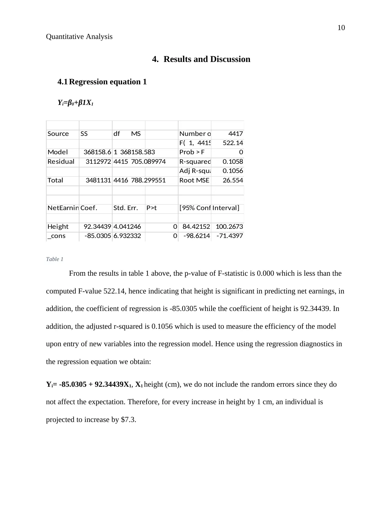
4.1 Regression equation 1
Yi=β0+β1X1
Source SS df MS Number of obs 4417
F( 1, 4415) 522.14
Model 368158.6 1 368158.583 Prob > F 0
Residual 3112972 4415 705.089974 R-squared 0.1058
Adj R-squared0.1056
Total 3481131 4416 788.299551 Root MSE 26.554
NetEarningCoef. Std. Err. tP>t [95% Conf.Interval]
Height 92.34439 4.041246 22.85 0 84.42152 100.2673
_cons -85.0305 6.932332 -12.27 0 -98.6214 -71.4397
Table 1
From the results in table 1 above, the p-value of F-statistic is 0.000 which is less than the
computed F-value 522.14, hence indicating that height is significant in predicting net earnings, in
addition, the coefficient of regression is -85.0305 while the coefficient of height is 92.34439. In
addition, the adjusted r-squared is 0.1056 which is used to measure the efficiency of the model
upon entry of new variables into the regression model. Hence using the regression diagnostics in
the regression equation we obtain:
Yi= -85.0305 + 92.34439X1, X1 height (cm), we do not include the random errors since they do
not affect the expectation. Therefore, for every increase in height by 1 cm, an individual is
projected to increase by $7.3.
Quantitative Analysis
4. Results and Discussion
4.1 Regression equation 1
Yi=β0+β1X1
Source SS df MS Number of obs 4417
F( 1, 4415) 522.14
Model 368158.6 1 368158.583 Prob > F 0
Residual 3112972 4415 705.089974 R-squared 0.1058
Adj R-squared0.1056
Total 3481131 4416 788.299551 Root MSE 26.554
NetEarningCoef. Std. Err. tP>t [95% Conf.Interval]
Height 92.34439 4.041246 22.85 0 84.42152 100.2673
_cons -85.0305 6.932332 -12.27 0 -98.6214 -71.4397
Table 1
From the results in table 1 above, the p-value of F-statistic is 0.000 which is less than the
computed F-value 522.14, hence indicating that height is significant in predicting net earnings, in
addition, the coefficient of regression is -85.0305 while the coefficient of height is 92.34439. In
addition, the adjusted r-squared is 0.1056 which is used to measure the efficiency of the model
upon entry of new variables into the regression model. Hence using the regression diagnostics in
the regression equation we obtain:
Yi= -85.0305 + 92.34439X1, X1 height (cm), we do not include the random errors since they do
not affect the expectation. Therefore, for every increase in height by 1 cm, an individual is
projected to increase by $7.3.
Paraphrase This Document
Need a fresh take? Get an instant paraphrase of this document with our AI Paraphraser
11
Quantitative Analysis
The p-value for the t-statistic is 0.000<0.05 at 95% confidence interval, we reject the null
hypothesis that height does not affect net earnings and conclude that there is significant evidence
that height affects net earnings, proving Pinsker (2015) correct.
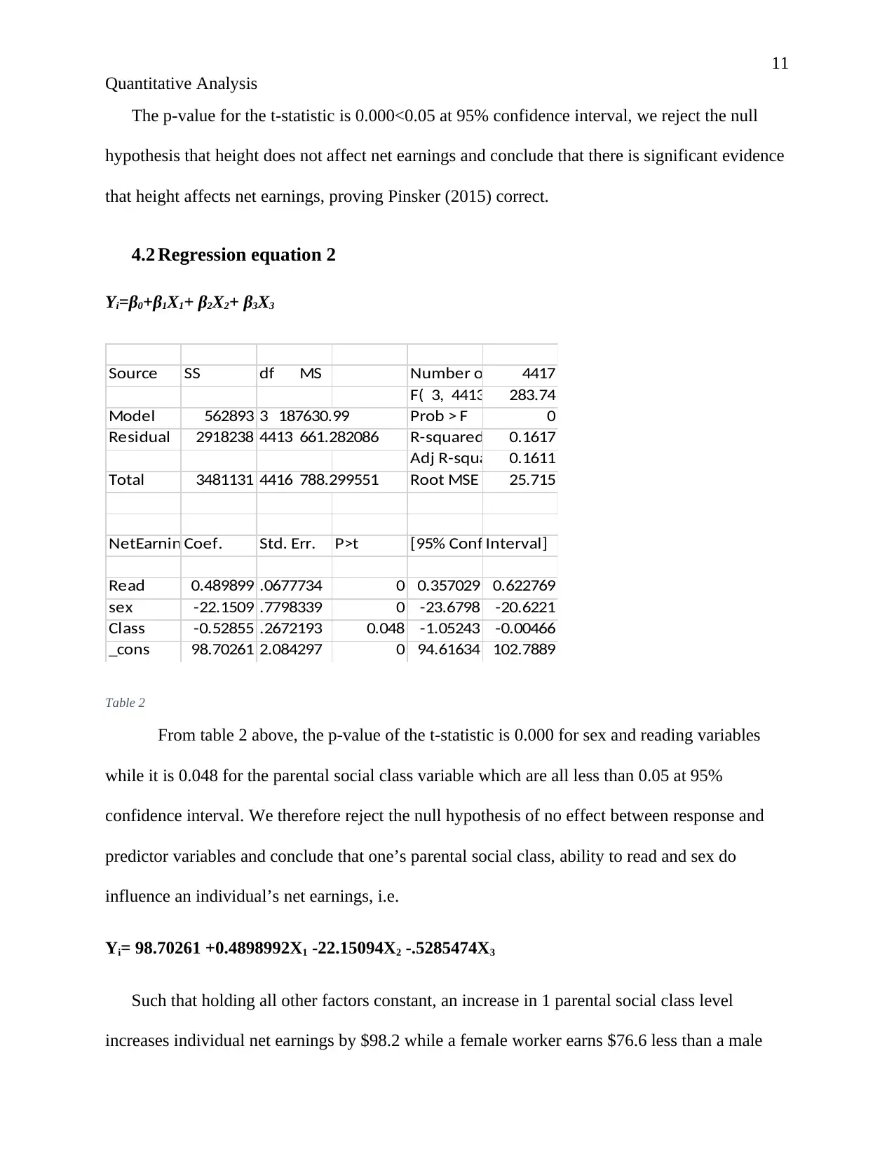
4.2 Regression equation 2
Yi=β0+β1X1+ β2X2+ β3X3
Source SS df MS Number of obs 4417
F( 3, 4413) 283.74
Model 562893 3 187630.99 Prob > F 0
Residual 2918238 4413 661.282086 R-squared 0.1617
Adj R-squared0.1611
Total 3481131 4416 788.299551 Root MSE 25.715
NetEarningCoef. Std. Err. tP>t [95% Conf.Interval]
Read 0.489899 .0677734 7.23 0 0.357029 0.622769
sex -22.1509 .7798339 -28.40 0 -23.6798 -20.6221
Class -0.52855 .2672193 -1.980.048 -1.05243 -0.00466
_cons 98.70261 2.084297 47.36 0 94.61634 102.7889
Table 2
From table 2 above, the p-value of the t-statistic is 0.000 for sex and reading variables
while it is 0.048 for the parental social class variable which are all less than 0.05 at 95%
confidence interval. We therefore reject the null hypothesis of no effect between response and
predictor variables and conclude that one’s parental social class, ability to read and sex do
influence an individual’s net earnings, i.e.
Yi= 98.70261 +0.4898992X1 -22.15094X2 -.5285474X3
Such that holding all other factors constant, an increase in 1 parental social class level
increases individual net earnings by $98.2 while a female worker earns $76.6 less than a male
Quantitative Analysis
The p-value for the t-statistic is 0.000<0.05 at 95% confidence interval, we reject the null
hypothesis that height does not affect net earnings and conclude that there is significant evidence
that height affects net earnings, proving Pinsker (2015) correct.
4.2 Regression equation 2
Yi=β0+β1X1+ β2X2+ β3X3
Source SS df MS Number of obs 4417
F( 3, 4413) 283.74
Model 562893 3 187630.99 Prob > F 0
Residual 2918238 4413 661.282086 R-squared 0.1617
Adj R-squared0.1611
Total 3481131 4416 788.299551 Root MSE 25.715
NetEarningCoef. Std. Err. tP>t [95% Conf.Interval]
Read 0.489899 .0677734 7.23 0 0.357029 0.622769
sex -22.1509 .7798339 -28.40 0 -23.6798 -20.6221
Class -0.52855 .2672193 -1.980.048 -1.05243 -0.00466
_cons 98.70261 2.084297 47.36 0 94.61634 102.7889
Table 2
From table 2 above, the p-value of the t-statistic is 0.000 for sex and reading variables
while it is 0.048 for the parental social class variable which are all less than 0.05 at 95%
confidence interval. We therefore reject the null hypothesis of no effect between response and
predictor variables and conclude that one’s parental social class, ability to read and sex do
influence an individual’s net earnings, i.e.
Yi= 98.70261 +0.4898992X1 -22.15094X2 -.5285474X3
Such that holding all other factors constant, an increase in 1 parental social class level
increases individual net earnings by $98.2 while a female worker earns $76.6 less than a male
12
Quantitative Analysis
worker. The ability of an individual to read has a positive relationship with net earnings where,
assuming that all other factors are constant one earns approximately $99.2 more than a person
who does not know how to read.
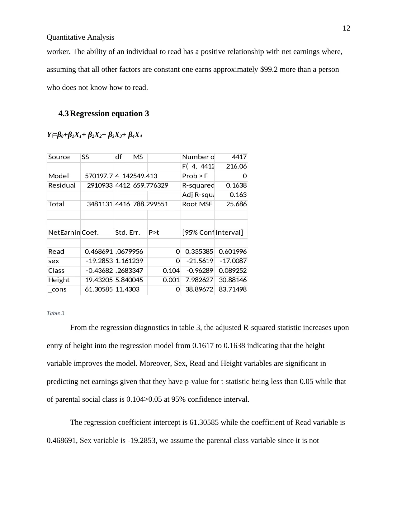
4.3 Regression equation 3
Yi=β0+β1X1+ β2X2+ β3X3+ β4X4
Source SS df MS Number of obs 4417
F( 4, 4412) 216.06
Model 570197.7 4 142549.413 Prob > F 0
Residual 2910933 4412 659.776329 R-squared 0.1638
Adj R-squared 0.163
Total 3481131 4416 788.299551 Root MSE 25.686
NetEarningCoef. Std. Err. tP>t [95% Conf.Interval]
Read 0.468691 .0679956 6.89 0 0.335385 0.601996
sex -19.2853 1.161239 -16.61 0 -21.5619 -17.0087
Class -0.43682 .2683347 -1.630.104 -0.96289 0.089252
Height 19.43205 5.840045 3.330.001 7.982627 30.88146
_cons 61.30585 11.4303 5.36 0 38.89672 83.71498
Table 3
From the regression diagnostics in table 3, the adjusted R-squared statistic increases upon
entry of height into the regression model from 0.1617 to 0.1638 indicating that the height
variable improves the model. Moreover, Sex, Read and Height variables are significant in
predicting net earnings given that they have p-value for t-statistic being less than 0.05 while that
of parental social class is 0.104>0.05 at 95% confidence interval.
The regression coefficient intercept is 61.30585 while the coefficient of Read variable is
0.468691, Sex variable is -19.2853, we assume the parental class variable since it is not
Quantitative Analysis
worker. The ability of an individual to read has a positive relationship with net earnings where,
assuming that all other factors are constant one earns approximately $99.2 more than a person
who does not know how to read.
4.3 Regression equation 3
Yi=β0+β1X1+ β2X2+ β3X3+ β4X4
Source SS df MS Number of obs 4417
F( 4, 4412) 216.06
Model 570197.7 4 142549.413 Prob > F 0
Residual 2910933 4412 659.776329 R-squared 0.1638
Adj R-squared 0.163
Total 3481131 4416 788.299551 Root MSE 25.686
NetEarningCoef. Std. Err. tP>t [95% Conf.Interval]
Read 0.468691 .0679956 6.89 0 0.335385 0.601996
sex -19.2853 1.161239 -16.61 0 -21.5619 -17.0087
Class -0.43682 .2683347 -1.630.104 -0.96289 0.089252
Height 19.43205 5.840045 3.330.001 7.982627 30.88146
_cons 61.30585 11.4303 5.36 0 38.89672 83.71498
Table 3
From the regression diagnostics in table 3, the adjusted R-squared statistic increases upon
entry of height into the regression model from 0.1617 to 0.1638 indicating that the height
variable improves the model. Moreover, Sex, Read and Height variables are significant in
predicting net earnings given that they have p-value for t-statistic being less than 0.05 while that
of parental social class is 0.104>0.05 at 95% confidence interval.
The regression coefficient intercept is 61.30585 while the coefficient of Read variable is
0.468691, Sex variable is -19.2853, we assume the parental class variable since it is not
⊘ This is a preview!⊘
Do you want full access?
Subscribe today to unlock all pages.
Trusted by 1+ million students worldwide
1 out of 16


Your All-in-One AI-Powered Toolkit for Academic Success.
+13062052269
info@desklib.com
Available 24*7 on WhatsApp / Email
![[object Object]](/_next/static/media/star-bottom.7253800d.svg)
Unlock your academic potential
Copyright © 2020–2026 A2Z Services. All Rights Reserved. Developed and managed by ZUCOL.