Schmeckt Gut: Economic Principles, Decision Making & Market Analysis
VerifiedAdded on 2023/06/10
|21
|5472
|258
Report
AI Summary
This report delves into the economic principles and decision-making processes surrounding Schmeckt Gut's planned market launch of the Schmeckt Besser energy bar in Atollia. It utilizes market analysis data provided by Schmeckt Gut's research department, focusing on scenarios involving varying income growth, inflation rates, and tariff rates on imports. The analysis employs a quantitative multiple regression approach to assess the sensitivity of product demand to changes in external economic variables. The report examines the relationship between macroeconomic indicators like income growth, inflation, and tariff rates, and their impact on the aggregate demand and supply. Furthermore, based on the regression analysis results, the report provides recommendations for Schmeckt Gut's management, considering different economic scenarios and their potential effects on the demand for the energy bar. The regression results highlight the significant influence of real income and tariffs on product demand, while the number of stores has a less significant impact. The report concludes with tailored strategies based on the projected economic conditions.
1
ECONOMICS PRINCIPLE AND DECISION MAKING
ECONOMICS PRINCIPLE AND DECISION MAKING
Paraphrase This Document
Need a fresh take? Get an instant paraphrase of this document with our AI Paraphraser
2
Executive summary
Decision making is crucial for any kind of business and market analysis works as a resource
for the process. Schmeckt Gut carries out market analysis and collects data based on the
demand for the product. The study in the paper uses the multiple regression analysis to find
out the effect of the dependent variable on the dependent variable. Furthermore, based on the
study and the relationship between the economic variables, the paper also presents
recommendations for the management of Schmeckt Gut.
3
Table of contents
1.0 Introduction..........................................................................................................................4
2.0 Methods................................................................................................................................4
3.0 Discussions...........................................................................................................................4
3.1 Relationship between the different projections....................................................................4
3.2 Impact on the demand for the product of the company.......................................................5
3.3 Recommendations................................................................................................................7
4.0 Conclusion............................................................................................................................9
Reference..................................................................................................................................10
⊘ This is a preview!⊘
Do you want full access?
Subscribe today to unlock all pages.
Trusted by 1+ million students worldwide
4
1.0 Introduction
Decision making is one of the important functions of any organisation. The decision making
becomes more crucial in the case of B2C businesses where the customers are the consumers
of the end products. There are few resources which are required for a company to make
decisions such as market analysis, survey and many more. In this study, Schmeckt Gut is a
company that wants to introduce its energy bar product in the market. Using its marketing
analysis result, this paper aims to discuss the impacts of the different economic variable on
the demand of the product. Based on that, the study carried out in the paper also presents
recommendations based on different situations.
2.0 Methods
The study carried out in the paper uses the data given by the marketing department of
Schmeckt Gut and the secondary data and information collected from other similar papers. A
quantitative multiple regression analysis has been carried out in the paper to arrive at the
result which shows the sensitivity of the demand of the product to the changes in the external
scenarios.
3.0 Discussions
3.1 Relationship between the different projections
The income growth and inflation are two of the most important macroeconomic indicators
that measure the performance of an economy. On the other hand, a tariff rate is a tool used by
the government in order to regulate the domestic market. Karlan (2017) stated that, lowered
tariff rate makes it easier for the foreign company to invade a domestic market which in turn
becomes a trouble for the indigenous businesses.
However, all the three values are dependent on each other. The direct relationship between
the income growth and the inflation rate is justified by the theory of demand and supply. As
the income grows at the rate of 1%, the consumers will demand more products from the
market and hence the demand curve will shift rightward leading to an increase in the price of
that specific product (Laibson & List, 2015). Now this increase in the price of the product,
over time, contributes to the degrading purchasing power of the consumer and hence the
inflation. Corresponding to a 1% increase in the income can result in either of inflation rate as
Paraphrase This Document
Need a fresh take? Get an instant paraphrase of this document with our AI Paraphraser
5
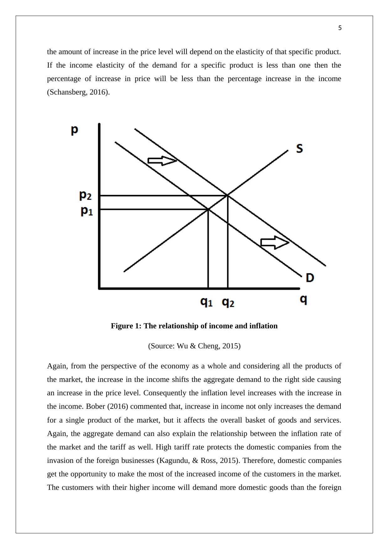
the amount of increase in the price level will depend on the elasticity of that specific product.
If the income elasticity of the demand for a specific product is less than one then the
percentage of increase in price will be less than the percentage increase in the income
(Schansberg, 2016).
Figure 1: The relationship of income and inflation
(Source: Wu & Cheng, 2015)
Again, from the perspective of the economy as a whole and considering all the products of
the market, the increase in the income shifts the aggregate demand to the right side causing
an increase in the price level. Consequently the inflation level increases with the increase in
the income. Bober (2016) commented that, increase in income not only increases the demand
for a single product of the market, but it affects the overall basket of goods and services.
Again, the aggregate demand can also explain the relationship between the inflation rate of
the market and the tariff as well. High tariff rate protects the domestic companies from the
invasion of the foreign businesses (Kagundu, & Ross, 2015). Therefore, domestic companies
get the opportunity to make the most of the increased income of the customers in the market.
The customers with their higher income will demand more domestic goods than the foreign
6
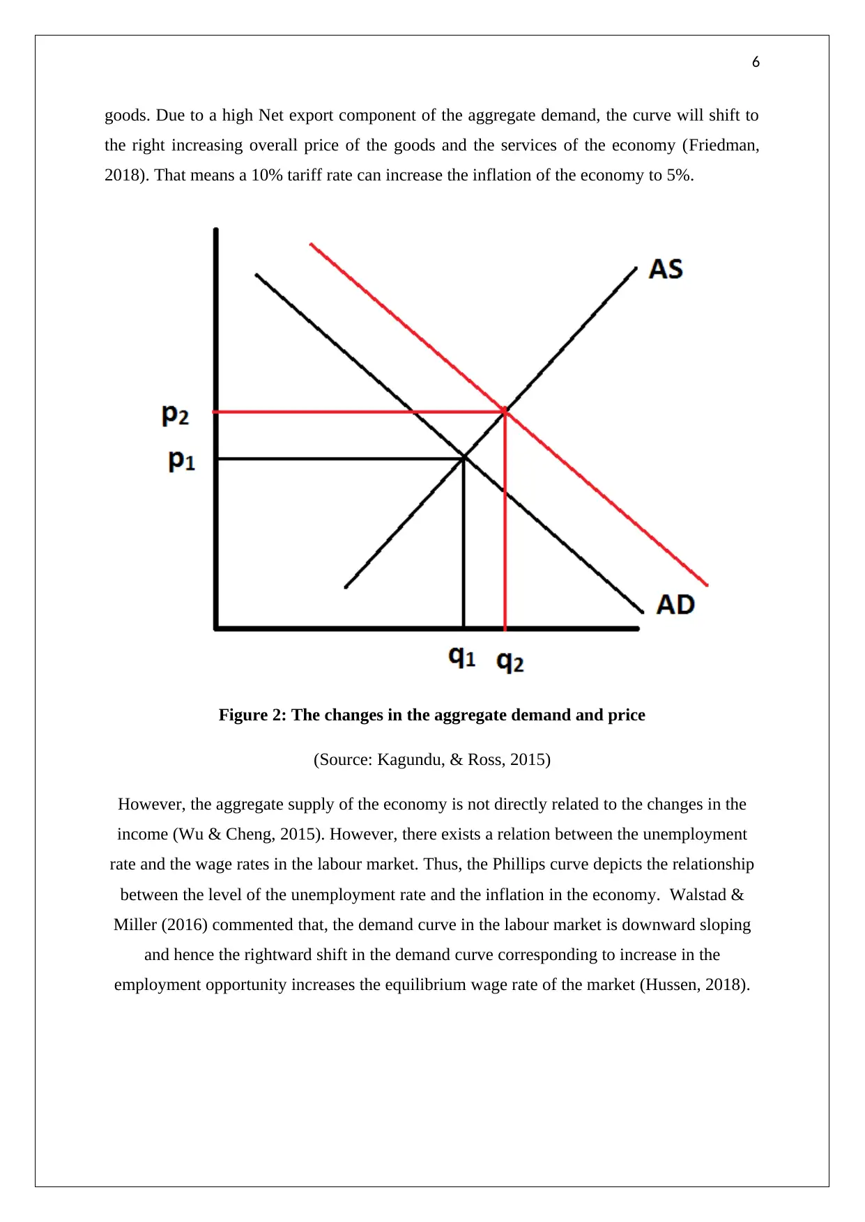
goods. Due to a high Net export component of the aggregate demand, the curve will shift to
the right increasing overall price of the goods and the services of the economy (Friedman,
2018). That means a 10% tariff rate can increase the inflation of the economy to 5%.
Figure 2: The changes in the aggregate demand and price
(Source: Kagundu, & Ross, 2015)
However, the aggregate supply of the economy is not directly related to the changes in the
income (Wu & Cheng, 2015). However, there exists a relation between the unemployment
rate and the wage rates in the labour market. Thus, the Phillips curve depicts the relationship
between the level of the unemployment rate and the inflation in the economy. Walstad &
Miller (2016) commented that, the demand curve in the labour market is downward sloping
and hence the rightward shift in the demand curve corresponding to increase in the
employment opportunity increases the equilibrium wage rate of the market (Hussen, 2018).
⊘ This is a preview!⊘
Do you want full access?
Subscribe today to unlock all pages.
Trusted by 1+ million students worldwide

7
Figure 3: Phillips curve
(Source: Hussen, 2018)
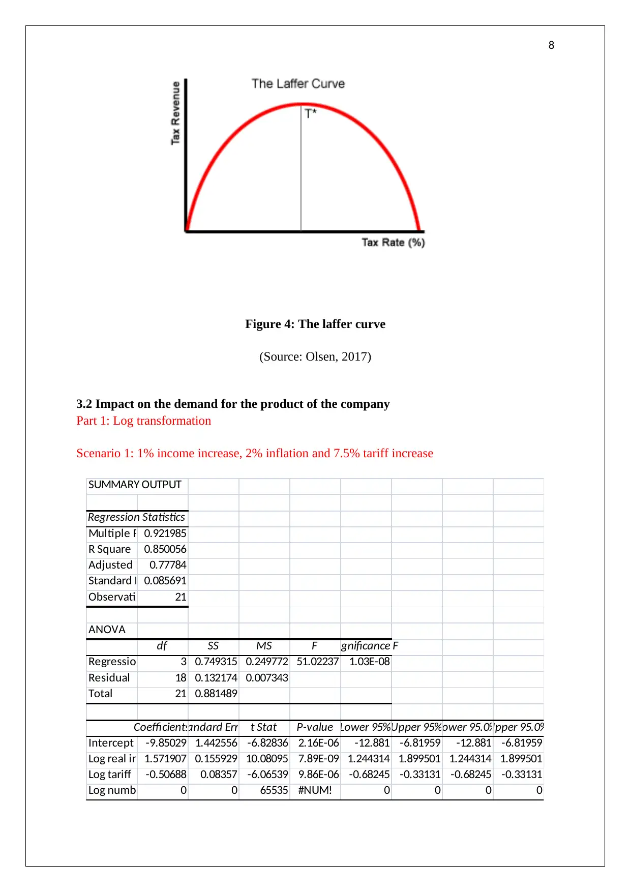
Lastly, the laffers curve shows the relationship between the amount of tax rate and total tax
revenue collected by the government. Gwartney, Stroup, Lee, Ferrarini & Calhoun (2016)
noted that, the government can increase the tax rate in order to increase the overall tax
revenue of the state. However, there is a limitation to the increase in the tax rate, as with
higher taxes, people will be discouraged to work. After a specific point, a higher tax reduces
the tax revenue of the government (Aljamal, Cader, Chiemeke & Speece, 2015). This is due
to the fact that, with high taxes the production of the economies goes down resulting in
deflation and stagnation in the economy.
Figure 3: Phillips curve
(Source: Hussen, 2018)
Lastly, the laffers curve shows the relationship between the amount of tax rate and total tax
revenue collected by the government. Gwartney, Stroup, Lee, Ferrarini & Calhoun (2016)
noted that, the government can increase the tax rate in order to increase the overall tax
revenue of the state. However, there is a limitation to the increase in the tax rate, as with
higher taxes, people will be discouraged to work. After a specific point, a higher tax reduces
the tax revenue of the government (Aljamal, Cader, Chiemeke & Speece, 2015). This is due
to the fact that, with high taxes the production of the economies goes down resulting in
deflation and stagnation in the economy.
Paraphrase This Document
Need a fresh take? Get an instant paraphrase of this document with our AI Paraphraser
8
Figure 4: The laffer curve
(Source: Olsen, 2017)
3.2 Impact on the demand for the product of the company
Part 1: Log transformation
Scenario 1: 1% income increase, 2% inflation and 7.5% tariff increase
SUMMARY OUTPUT
Regression Statistics
Multiple R 0.921985
R Square 0.850056
Adjusted R Square0.77784
Standard Error0.085691
Observations 21
ANOVA
df SS MS F Significance F
Regression 3 0.749315 0.249772 51.02237 1.03E-08
Residual 18 0.132174 0.007343
Total 21 0.881489
CoefficientsStandard Error t Stat P-value Lower 95%Upper 95%Lower 95.0%Upper 95.0%
Intercept -9.85029 1.442556 -6.82836 2.16E-06 -12.881 -6.81959 -12.881 -6.81959
Log real income1.571907 0.155929 10.08095 7.89E-09 1.244314 1.899501 1.244314 1.899501
Log tariff -0.50688 0.08357 -6.06539 9.86E-06 -0.68245 -0.33131 -0.68245 -0.33131
Log number of stores0 0 65535 #NUM! 0 0 0 0
9
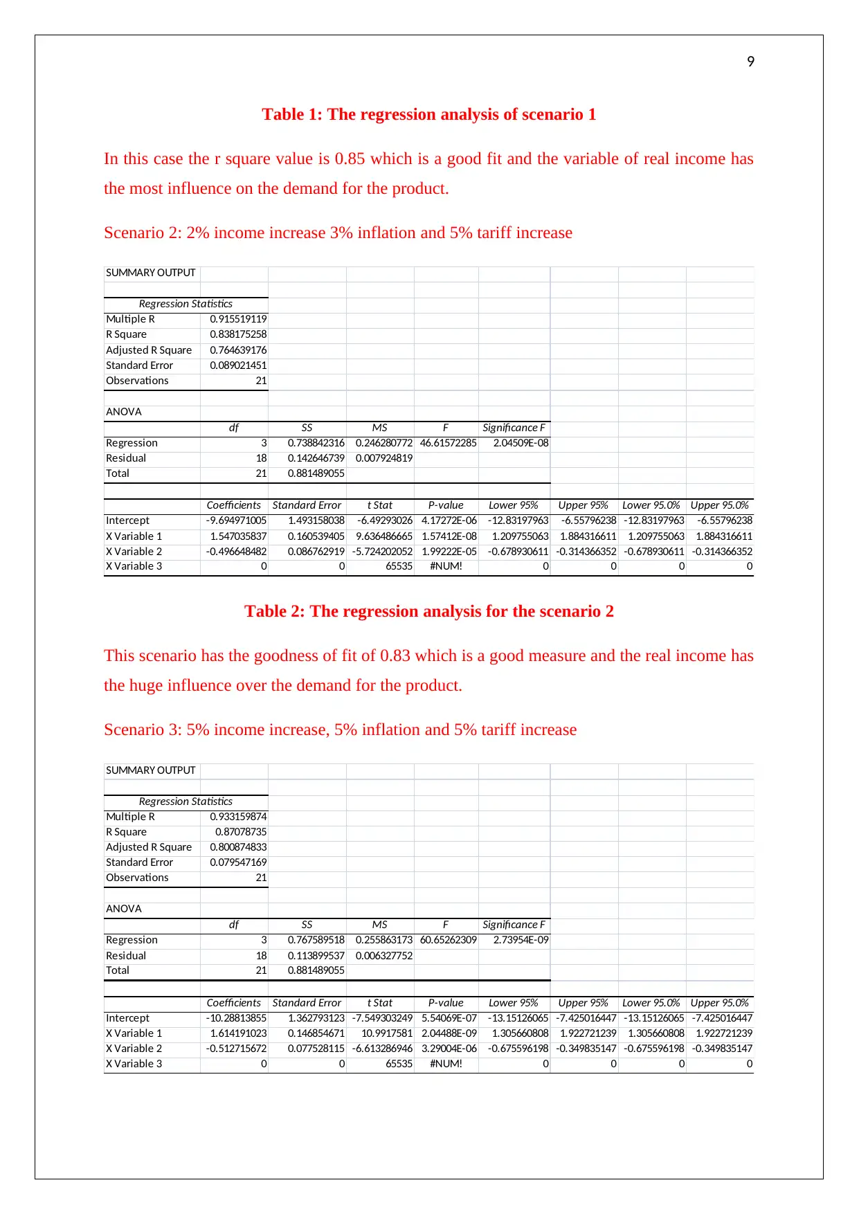
Table 1: The regression analysis of scenario 1
In this case the r square value is 0.85 which is a good fit and the variable of real income has
the most influence on the demand for the product.
Scenario 2: 2% income increase 3% inflation and 5% tariff increase
SUMMARY OUTPUT
Regression Statistics
Multiple R 0.915519119
R Square 0.838175258
Adjusted R Square 0.764639176
Standard Error 0.089021451
Observations 21
ANOVA
df SS MS F Significance F
Regression 3 0.738842316 0.246280772 46.61572285 2.04509E-08
Residual 18 0.142646739 0.007924819
Total 21 0.881489055
Coefficients Standard Error t Stat P-value Lower 95% Upper 95% Lower 95.0% Upper 95.0%
Intercept -9.694971005 1.493158038 -6.49293026 4.17272E-06 -12.83197963 -6.55796238 -12.83197963 -6.55796238
X Variable 1 1.547035837 0.160539405 9.636486665 1.57412E-08 1.209755063 1.884316611 1.209755063 1.884316611
X Variable 2 -0.496648482 0.086762919 -5.724202052 1.99222E-05 -0.678930611 -0.314366352 -0.678930611 -0.314366352
X Variable 3 0 0 65535 #NUM! 0 0 0 0
Table 2: The regression analysis for the scenario 2
This scenario has the goodness of fit of 0.83 which is a good measure and the real income has
the huge influence over the demand for the product.
Scenario 3: 5% income increase, 5% inflation and 5% tariff increase
SUMMARY OUTPUT
Regression Statistics
Multiple R 0.933159874
R Square 0.87078735
Adjusted R Square 0.800874833
Standard Error 0.079547169
Observations 21
ANOVA
df SS MS F Significance F
Regression 3 0.767589518 0.255863173 60.65262309 2.73954E-09
Residual 18 0.113899537 0.006327752
Total 21 0.881489055
Coefficients Standard Error t Stat P-value Lower 95% Upper 95% Lower 95.0% Upper 95.0%
Intercept -10.28813855 1.362793123 -7.549303249 5.54069E-07 -13.15126065 -7.425016447 -13.15126065 -7.425016447
X Variable 1 1.614191023 0.146854671 10.9917581 2.04488E-09 1.305660808 1.922721239 1.305660808 1.922721239
X Variable 2 -0.512715672 0.077528115 -6.613286946 3.29004E-06 -0.675596198 -0.349835147 -0.675596198 -0.349835147
X Variable 3 0 0 65535 #NUM! 0 0 0 0
⊘ This is a preview!⊘
Do you want full access?
Subscribe today to unlock all pages.
Trusted by 1+ million students worldwide
10
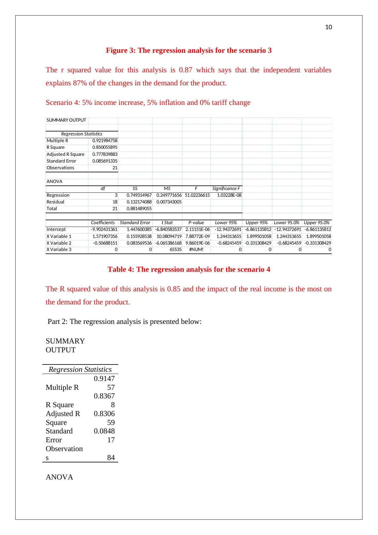
Figure 3: The regression analysis for the scenario 3
The r squared value for this analysis is 0.87 which says that the independent variables
explains 87% of the changes in the demand for the product.
Scenario 4: 5% income increase, 5% inflation and 0% tariff change
SUMMARY OUTPUT
Regression Statistics
Multiple R 0.921984758
R Square 0.850055895
Adjusted R Square 0.777839883
Standard Error 0.085691335
Observations 21
ANOVA
df SS MS F Significance F
Regression 3 0.749314967 0.249771656 51.02236615 1.03228E-08
Residual 18 0.132174088 0.007343005
Total 21 0.881489055
Coefficients Standard Error t Stat P-value Lower 95% Upper 95% Lower 95.0% Upper 95.0%
Intercept -9.902431361 1.447600385 -6.840583537 2.11151E-06 -12.94372691 -6.861135812 -12.94372691 -6.861135812
X Variable 1 1.571907356 0.155928538 10.08094719 7.88772E-09 1.244313655 1.899501058 1.244313655 1.899501058
X Variable 2 -0.50688151 0.083569536 -6.065386168 9.86019E-06 -0.68245459 -0.331308429 -0.68245459 -0.331308429
X Variable 3 0 0 65535 #NUM! 0 0 0 0
Table 4: The regression analysis for the scenario 4
The R squared value of this analysis is 0.85 and the impact of the real income is the most on
the demand for the product.
Part 2: The regression analysis is presented below:
SUMMARY
OUTPUT
Regression Statistics
Multiple R
0.9147
57
R Square
0.8367
8
Adjusted R
Square
0.8306
59
Standard
Error
0.0848
17
Observation
s 84
ANOVA
Paraphrase This Document
Need a fresh take? Get an instant paraphrase of this document with our AI Paraphraser
11
df SS MS F
Signific
ance F
Regression 3 2.950449
0.983
483
136.7
118
2.14E-
31
Residual 80 0.575507
0.007
194
Total 83 3.525956
Coeffic
ients
Standard
Error t Stat
P-
value
Lower
95%
Upper
95%
Lower
95.0%
Upper
95.0%
Intercept
-
9.5375
9 0.721743
-
13.21
47
8.24
E-22
-
10.9739
-
8.1012
7
-
10.9739
-
8.10127
Log real
income
1.5471
33 0.076553
20.21
008
3.61
E-33
1.39478
8
1.6994
77
1.39478
8
1.69947
7
Log tariff
-
0.4936
1 0.041094
-
12.01
19
1.36
E-19
-
0.57539
-
0.4118
3
-
0.57539
-
0.41183
Log number
of stores
-
0.0452
9 0.054189
-
0.835
71
0.405
809
-
0.15313
0.0625
54
-
0.15313
0.06255
4
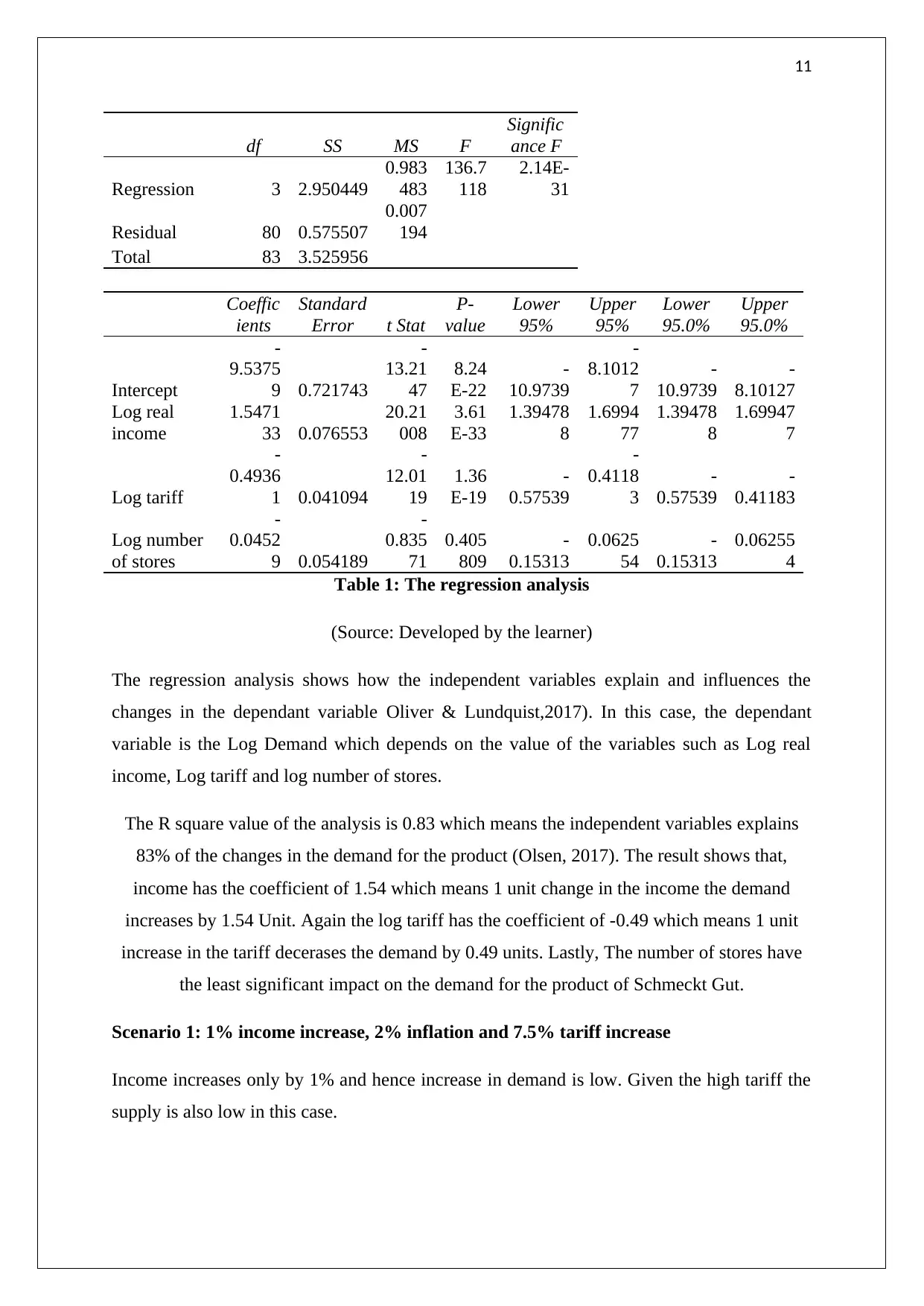
Table 1: The regression analysis
(Source: Developed by the learner)
The regression analysis shows how the independent variables explain and influences the
changes in the dependant variable Oliver & Lundquist,2017). In this case, the dependant
variable is the Log Demand which depends on the value of the variables such as Log real
income, Log tariff and log number of stores.
The R square value of the analysis is 0.83 which means the independent variables explains
83% of the changes in the demand for the product (Olsen, 2017). The result shows that,
income has the coefficient of 1.54 which means 1 unit change in the income the demand
increases by 1.54 Unit. Again the log tariff has the coefficient of -0.49 which means 1 unit
increase in the tariff decerases the demand by 0.49 units. Lastly, The number of stores have
the least significant impact on the demand for the product of Schmeckt Gut.
Scenario 1: 1% income increase, 2% inflation and 7.5% tariff increase
Income increases only by 1% and hence increase in demand is low. Given the high tariff the
supply is also low in this case.
df SS MS F
Signific
ance F
Regression 3 2.950449
0.983
483
136.7
118
2.14E-
31
Residual 80 0.575507
0.007
194
Total 83 3.525956
Coeffic
ients
Standard
Error t Stat
P-
value
Lower
95%
Upper
95%
Lower
95.0%
Upper
95.0%
Intercept
-
9.5375
9 0.721743
-
13.21
47
8.24
E-22
-
10.9739
-
8.1012
7
-
10.9739
-
8.10127
Log real
income
1.5471
33 0.076553
20.21
008
3.61
E-33
1.39478
8
1.6994
77
1.39478
8
1.69947
7
Log tariff
-
0.4936
1 0.041094
-
12.01
19
1.36
E-19
-
0.57539
-
0.4118
3
-
0.57539
-
0.41183
Log number
of stores
-
0.0452
9 0.054189
-
0.835
71
0.405
809
-
0.15313
0.0625
54
-
0.15313
0.06255
4
Table 1: The regression analysis
(Source: Developed by the learner)
The regression analysis shows how the independent variables explain and influences the
changes in the dependant variable Oliver & Lundquist,2017). In this case, the dependant
variable is the Log Demand which depends on the value of the variables such as Log real
income, Log tariff and log number of stores.
The R square value of the analysis is 0.83 which means the independent variables explains
83% of the changes in the demand for the product (Olsen, 2017). The result shows that,
income has the coefficient of 1.54 which means 1 unit change in the income the demand
increases by 1.54 Unit. Again the log tariff has the coefficient of -0.49 which means 1 unit
increase in the tariff decerases the demand by 0.49 units. Lastly, The number of stores have
the least significant impact on the demand for the product of Schmeckt Gut.
Scenario 1: 1% income increase, 2% inflation and 7.5% tariff increase
Income increases only by 1% and hence increase in demand is low. Given the high tariff the
supply is also low in this case.
12
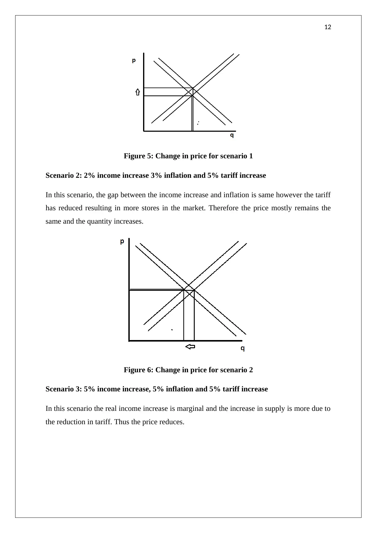
Figure 5: Change in price for scenario 1
Scenario 2: 2% income increase 3% inflation and 5% tariff increase
In this scenario, the gap between the income increase and inflation is same however the tariff
has reduced resulting in more stores in the market. Therefore the price mostly remains the
same and the quantity increases.
Figure 6: Change in price for scenario 2
Scenario 3: 5% income increase, 5% inflation and 5% tariff increase
In this scenario the real income increase is marginal and the increase in supply is more due to
the reduction in tariff. Thus the price reduces.
⊘ This is a preview!⊘
Do you want full access?
Subscribe today to unlock all pages.
Trusted by 1+ million students worldwide
1 out of 21
Related Documents


Your All-in-One AI-Powered Toolkit for Academic Success.
+13062052269
info@desklib.com
Available 24*7 on WhatsApp / Email
![[object Object]](/_next/static/media/star-bottom.7253800d.svg)
Unlock your academic potential
Copyright © 2020–2026 A2Z Services. All Rights Reserved. Developed and managed by ZUCOL.