Scientific Report on BMI, TEE, Statistical Analysis, and Correlation
VerifiedAdded on 2022/12/28
|18
|3255
|21
Report
AI Summary
This scientific report presents an analysis of body mass index (BMI) and total energy expenditure (TEE). The study investigates the relationship between these variables using statistical methods, including t-tests to determine the significance of data between Group A and Group B. The report details the methods used, such as statistical analysis and correlation, to explore the connection between the two groups and assess any significant differences. It covers key aspects of TEE, including physical activity energy expenditure, resting energy expenditure, and resting metabolic rate (RMR). The objective is to estimate TEE, forecast RMR, and assess physical activity levels (PAL) through physical activity diaries and compendiums. The report also discusses the calculation of P-values, statistical analysis, and correlation, offering insights into the significance of the findings and the relationships between variables such as body weight, physical activity, and RMR. Furthermore, metabolic equivalents (MET) are discussed in relation to activity levels and energy expenditure.

Scientific Report Writing
1
1
Paraphrase This Document
Need a fresh take? Get an instant paraphrase of this document with our AI Paraphraser
ABSTRACT
The study summaries scientific analysis of body mass index and total TEE for both group as
well as connection with total energy expenditure is discussed. By performing T Test P values for
Group A and Group B in the context of BMI are determined which help to assess the actual
significance of data. Further the study comprises certain major methods like statistical analysis,
correlation etc. which clearly states the relationship between two group and also support in
determining the significance difference to better explore the relevance of study.
2
Contents
ABSTRACT.....................................................................................................................................2
Contents...........................................................................................................................................3
Introduction and Aim.......................................................................................................................4
Methods and Discussion..................................................................................................................4
Conclusion.....................................................................................................................................12
REFERENCES..............................................................................................................................13
Appendix........................................................................................................................................14
3
⊘ This is a preview!⊘
Do you want full access?
Subscribe today to unlock all pages.
Trusted by 1+ million students worldwide
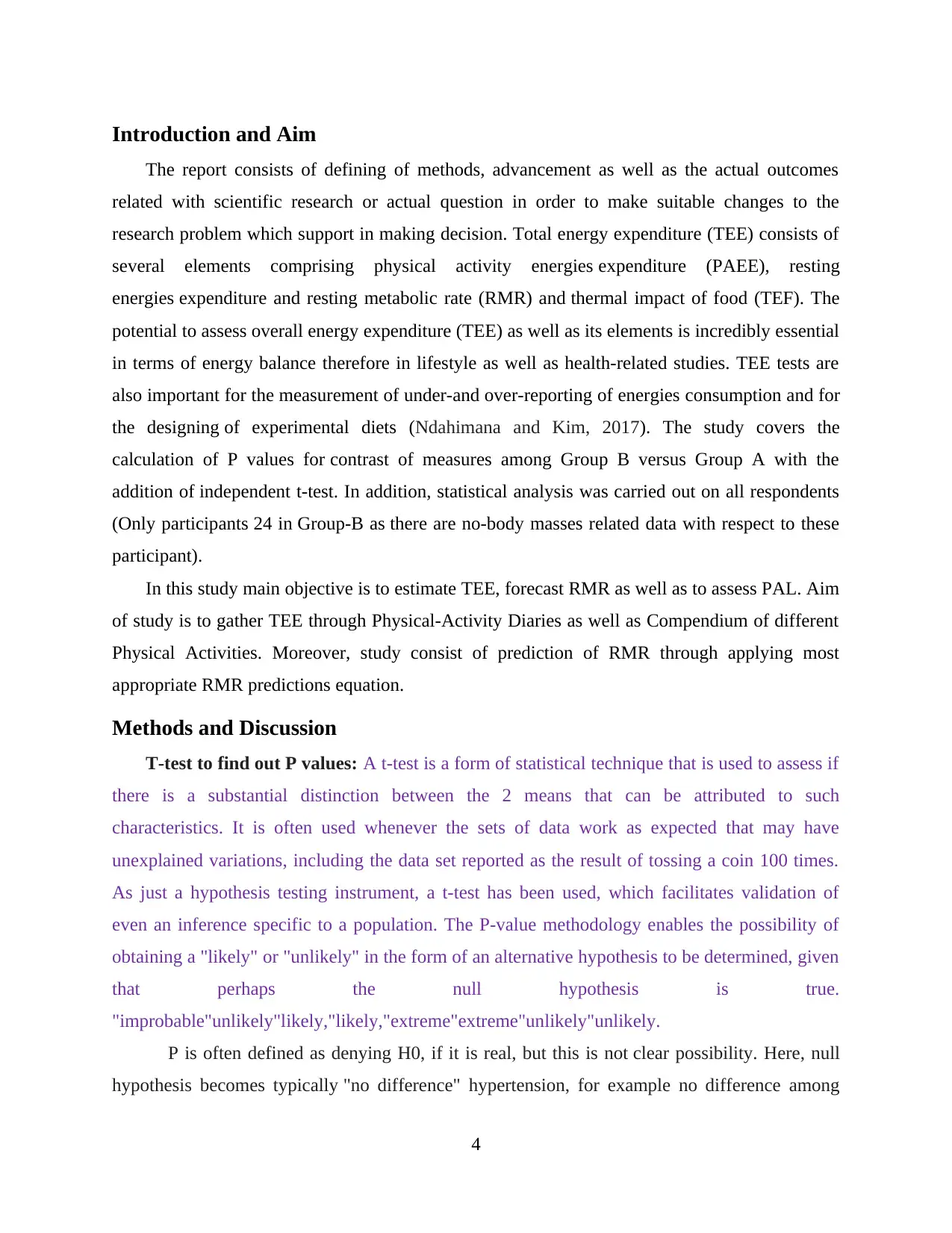
Introduction and Aim
The report consists of defining of methods, advancement as well as the actual outcomes
related with scientific research or actual question in order to make suitable changes to the
research problem which support in making decision. Total energy expenditure (TEE) consists of
several elements comprising physical activity energies expenditure (PAEE), resting
energies expenditure and resting metabolic rate (RMR) and thermal impact of food (TEF). The
potential to assess overall energy expenditure (TEE) as well as its elements is incredibly essential
in terms of energy balance therefore in lifestyle as well as health-related studies. TEE tests are
also important for the measurement of under-and over-reporting of energies consumption and for
the designing of experimental diets (Ndahimana and Kim, 2017). The study covers the
calculation of P values for contrast of measures among Group B versus Group A with the
addition of independent t-test. In addition, statistical analysis was carried out on all respondents
(Only participants 24 in Group-B as there are no-body masses related data with respect to these
participant).
In this study main objective is to estimate TEE, forecast RMR as well as to assess PAL. Aim
of study is to gather TEE through Physical-Activity Diaries as well as Compendium of different
Physical Activities. Moreover, study consist of prediction of RMR through applying most
appropriate RMR predictions equation.
Methods and Discussion
T-test to find out P values: A t-test is a form of statistical technique that is used to assess if
there is a substantial distinction between the 2 means that can be attributed to such
characteristics. It is often used whenever the sets of data work as expected that may have
unexplained variations, including the data set reported as the result of tossing a coin 100 times.
As just a hypothesis testing instrument, a t-test has been used, which facilitates validation of
even an inference specific to a population. The P-value methodology enables the possibility of
obtaining a "likely" or "unlikely" in the form of an alternative hypothesis to be determined, given
that perhaps the null hypothesis is true.
"improbable"unlikely"likely,"likely,"extreme"extreme"unlikely"unlikely.
P is often defined as denying H0, if it is real, but this is not clear possibility. Here, null
hypothesis becomes typically "no difference" hypertension, for example no difference among
4
Paraphrase This Document
Need a fresh take? Get an instant paraphrase of this document with our AI Paraphraser
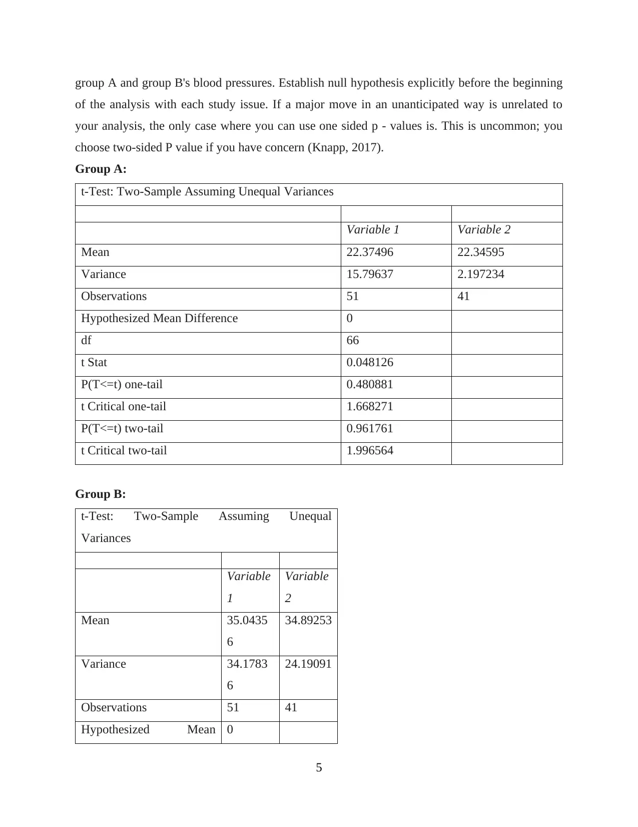
group A and group B's blood pressures. Establish null hypothesis explicitly before the beginning
of the analysis with each study issue. If a major move in an unanticipated way is unrelated to
your analysis, the only case where you can use one sided p - values is. This is uncommon; you
choose two-sided P value if you have concern (Knapp, 2017).
Group A:
t-Test: Two-Sample Assuming Unequal Variances
Variable 1 Variable 2
Mean 22.37496 22.34595
Variance 15.79637 2.197234
Observations 51 41
Hypothesized Mean Difference 0
df 66
t Stat 0.048126
P(T<=t) one-tail 0.480881
t Critical one-tail 1.668271
P(T<=t) two-tail 0.961761
t Critical two-tail 1.996564
Group B:
t-Test: Two-Sample Assuming Unequal
Variances
Variable
1
Variable
2
Mean 35.0435
6
34.89253
Variance 34.1783
6
24.19091
Observations 51 41
Hypothesized Mean 0
5
Difference
df 90
t Stat 0.13453
5
P(T<=t) one-tail 0.44664
t Critical one-tail 1.66196
1
P(T<=t) two-tail 0.89328
t Critical two-tail 1.98667
5
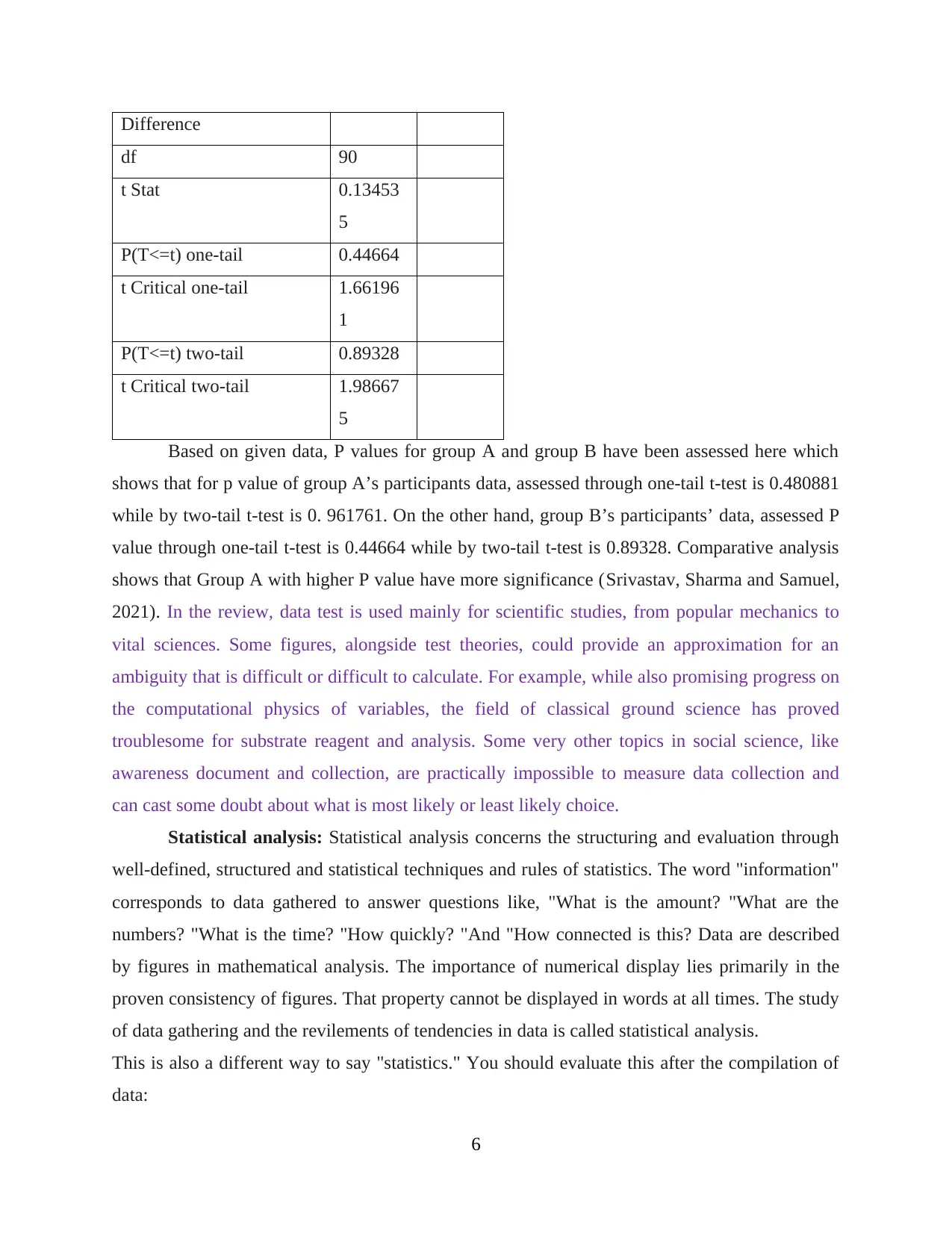
Based on given data, P values for group A and group B have been assessed here which
shows that for p value of group A’s participants data, assessed through one-tail t-test is 0.480881
while by two-tail t-test is 0. 961761. On the other hand, group B’s participants’ data, assessed P
value through one-tail t-test is 0.44664 while by two-tail t-test is 0.89328. Comparative analysis
shows that Group A with higher P value have more significance (Srivastav, Sharma and Samuel,
2021). In the review, data test is used mainly for scientific studies, from popular mechanics to
vital sciences. Some figures, alongside test theories, could provide an approximation for an
ambiguity that is difficult or difficult to calculate. For example, while also promising progress on
the computational physics of variables, the field of classical ground science has proved
troublesome for substrate reagent and analysis. Some very other topics in social science, like
awareness document and collection, are practically impossible to measure data collection and
can cast some doubt about what is most likely or least likely choice.
Statistical analysis: Statistical analysis concerns the structuring and evaluation through
well-defined, structured and statistical techniques and rules of statistics. The word "information"
corresponds to data gathered to answer questions like, "What is the amount? "What are the
numbers? "What is the time? "How quickly? "And "How connected is this? Data are described
by figures in mathematical analysis. The importance of numerical display lies primarily in the
proven consistency of figures. That property cannot be displayed in words at all times. The study
of data gathering and the revilements of tendencies in data is called statistical analysis.
This is also a different way to say "statistics." You should evaluate this after the compilation of
data:
6
df 90
t Stat 0.13453
5
P(T<=t) one-tail 0.44664
t Critical one-tail 1.66196
1
P(T<=t) two-tail 0.89328
t Critical two-tail 1.98667
5
Based on given data, P values for group A and group B have been assessed here which
shows that for p value of group A’s participants data, assessed through one-tail t-test is 0.480881
while by two-tail t-test is 0. 961761. On the other hand, group B’s participants’ data, assessed P
value through one-tail t-test is 0.44664 while by two-tail t-test is 0.89328. Comparative analysis
shows that Group A with higher P value have more significance (Srivastav, Sharma and Samuel,
2021). In the review, data test is used mainly for scientific studies, from popular mechanics to
vital sciences. Some figures, alongside test theories, could provide an approximation for an
ambiguity that is difficult or difficult to calculate. For example, while also promising progress on
the computational physics of variables, the field of classical ground science has proved
troublesome for substrate reagent and analysis. Some very other topics in social science, like
awareness document and collection, are practically impossible to measure data collection and
can cast some doubt about what is most likely or least likely choice.
Statistical analysis: Statistical analysis concerns the structuring and evaluation through
well-defined, structured and statistical techniques and rules of statistics. The word "information"
corresponds to data gathered to answer questions like, "What is the amount? "What are the
numbers? "What is the time? "How quickly? "And "How connected is this? Data are described
by figures in mathematical analysis. The importance of numerical display lies primarily in the
proven consistency of figures. That property cannot be displayed in words at all times. The study
of data gathering and the revilements of tendencies in data is called statistical analysis.
This is also a different way to say "statistics." You should evaluate this after the compilation of
data:
6
⊘ This is a preview!⊘
Do you want full access?
Subscribe today to unlock all pages.
Trusted by 1+ million students worldwide
Completely summarise all the given data. Create a pie map, for starters.
Search the main location steps. For starters, the medium informs the average number of
given data set.
Determine scatter values, which show whether data is clustered or scattered closer. The
default variance is one of the most widely used spread measures; it shows how average
spread of data is.
Create predictions for future cantered on previous behaviour. In retail, produce,
insurance, athletics or some other organisation, this is particularly useful because it
profits from knowing future patterns (Yulianti, 2017).
Testing the hypothesis in experiments. When you evaluate the results, gathering
information from experiment just reveals a story. Throughout this section, the figures are
officially referred to as "Hypothesis Testing," which either demonstrates or refutes null
hypothesis (the popular theory) (Guetterman, 2019).
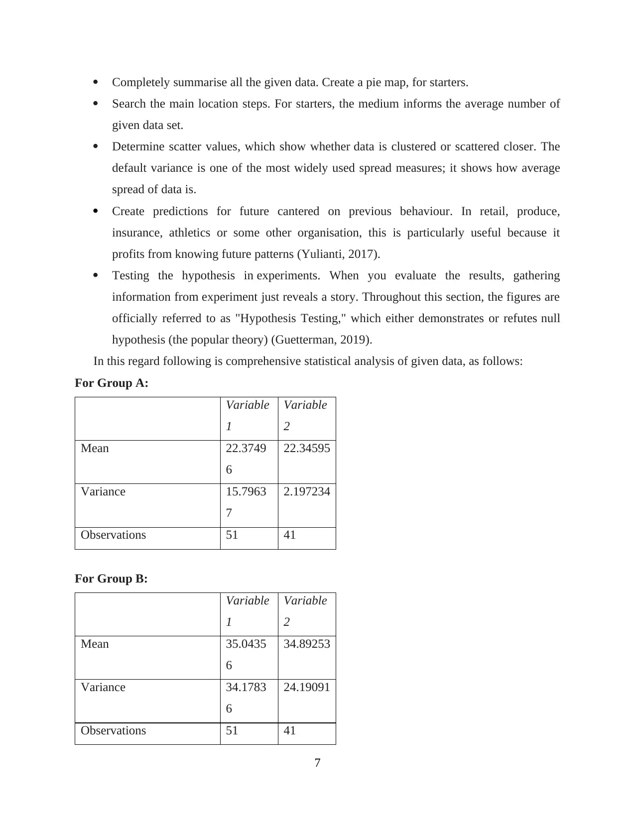
In this regard following is comprehensive statistical analysis of given data, as follows:
For Group A:
Variable
1
Variable
2
Mean 22.3749
6
22.34595
Variance 15.7963
7
2.197234
Observations 51 41
For Group B:
Variable
1
Variable
2
Mean 35.0435
6
34.89253
Variance 34.1783
6
24.19091
Observations 51 41
7
Search the main location steps. For starters, the medium informs the average number of
given data set.
Determine scatter values, which show whether data is clustered or scattered closer. The
default variance is one of the most widely used spread measures; it shows how average
spread of data is.
Create predictions for future cantered on previous behaviour. In retail, produce,
insurance, athletics or some other organisation, this is particularly useful because it
profits from knowing future patterns (Yulianti, 2017).
Testing the hypothesis in experiments. When you evaluate the results, gathering
information from experiment just reveals a story. Throughout this section, the figures are
officially referred to as "Hypothesis Testing," which either demonstrates or refutes null
hypothesis (the popular theory) (Guetterman, 2019).
In this regard following is comprehensive statistical analysis of given data, as follows:
For Group A:
Variable
1
Variable
2
Mean 22.3749
6
22.34595
Variance 15.7963
7
2.197234
Observations 51 41
For Group B:
Variable
1
Variable
2
Mean 35.0435
6
34.89253
Variance 34.1783
6
24.19091
Observations 51 41
7
Paraphrase This Document
Need a fresh take? Get an instant paraphrase of this document with our AI Paraphraser
Above analysis for Group A and B shows that Mean value of Group A for variable 1 is
22.37 and for variable 2 is 22.34 respectively. While with respect to Group B mean of variable 1
is 35.04 and of variable 2 is 34.89. At a constant rotational speed, the device pulls air thru the
bonnet and tests the proportion of depleted CO2 (FECO2) and O2 (FEO2) and then calculates
the fuel absorption rate (V-cit O2) and also the rate for greenhouse gases (V-cit CO2). These V-
circulated O2 and V-circulated CO2 levels have been used, utilizing implicit gravimetric
formulas, to calculate high carb oxidation levels and energy usage rates. RMR yield similar
results offer a practical alternative to implicit gravimetric RMR calculations, given recognized
disadvantages, as certain energy demands can be calculated using regularly available variables
like weight, gender, age and size. The spending on iterative solution equipment, the need for
trained personnel and the time-consuming nature of the RMR measurement preclude the periodic
supply of iterative solution devices.
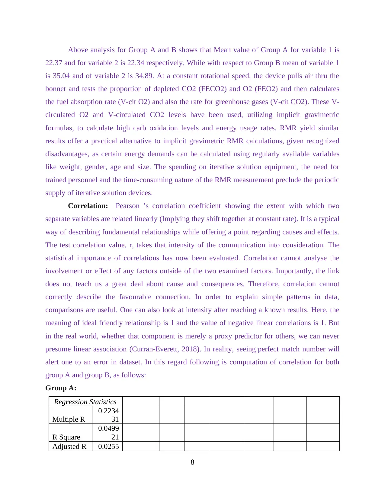
Correlation: Pearson ’s correlation coefficient showing the extent with which two
separate variables are related linearly (Implying they shift together at constant rate). It is a typical
way of describing fundamental relationships while offering a point regarding causes and effects.
The test correlation value, r, takes that intensity of the communication into consideration. The
statistical importance of correlations has now been evaluated. Correlation cannot analyse the
involvement or effect of any factors outside of the two examined factors. Importantly, the link
does not teach us a great deal about cause and consequences. Therefore, correlation cannot
correctly describe the favourable connection. In order to explain simple patterns in data,
comparisons are useful. One can also look at intensity after reaching a known results. Here, the
meaning of ideal friendly relationship is 1 and the value of negative linear correlations is 1. But
in the real world, whether that component is merely a proxy predictor for others, we can never
presume linear association (Curran-Everett, 2018). In reality, seeing perfect match number will
alert one to an error in dataset. In this regard following is computation of correlation for both
group A and group B, as follows:
Group A:
Regression Statistics
Multiple R
0.2234
31
R Square
0.0499
21
Adjusted R 0.0255
8
22.37 and for variable 2 is 22.34 respectively. While with respect to Group B mean of variable 1
is 35.04 and of variable 2 is 34.89. At a constant rotational speed, the device pulls air thru the
bonnet and tests the proportion of depleted CO2 (FECO2) and O2 (FEO2) and then calculates
the fuel absorption rate (V-cit O2) and also the rate for greenhouse gases (V-cit CO2). These V-
circulated O2 and V-circulated CO2 levels have been used, utilizing implicit gravimetric
formulas, to calculate high carb oxidation levels and energy usage rates. RMR yield similar
results offer a practical alternative to implicit gravimetric RMR calculations, given recognized
disadvantages, as certain energy demands can be calculated using regularly available variables
like weight, gender, age and size. The spending on iterative solution equipment, the need for
trained personnel and the time-consuming nature of the RMR measurement preclude the periodic
supply of iterative solution devices.
Correlation: Pearson ’s correlation coefficient showing the extent with which two
separate variables are related linearly (Implying they shift together at constant rate). It is a typical
way of describing fundamental relationships while offering a point regarding causes and effects.
The test correlation value, r, takes that intensity of the communication into consideration. The
statistical importance of correlations has now been evaluated. Correlation cannot analyse the
involvement or effect of any factors outside of the two examined factors. Importantly, the link
does not teach us a great deal about cause and consequences. Therefore, correlation cannot
correctly describe the favourable connection. In order to explain simple patterns in data,
comparisons are useful. One can also look at intensity after reaching a known results. Here, the
meaning of ideal friendly relationship is 1 and the value of negative linear correlations is 1. But
in the real world, whether that component is merely a proxy predictor for others, we can never
presume linear association (Curran-Everett, 2018). In reality, seeing perfect match number will
alert one to an error in dataset. In this regard following is computation of correlation for both
group A and group B, as follows:
Group A:
Regression Statistics
Multiple R
0.2234
31
R Square
0.0499
21
Adjusted R 0.0255
8
Square 61
Standard
Error
3.8932
5
Observatio
ns 41
ANOVA
df SS MS F
Significa
nce F
Regression 1 31.06114
31.06
114
2.049
239
0.16024
8
Residual 39 591.1385
15.15
74
Total 40 622.1996
Coeffic
ients
Standard
Error t Stat
P-
value
Lower
95%
Upper
95%
Lower
95.0%
Upper
95.0%
Intercept
8.9760
08 9.299791
0.965
184
0.340
4 -9.83459
27.786
61
-
9.83459
27.7866
1
X Variable
1
0.5944
84 0.415283
1.431
516
0.160
248 -0.2455
1.4344
74 -0.2455
1.43447
4
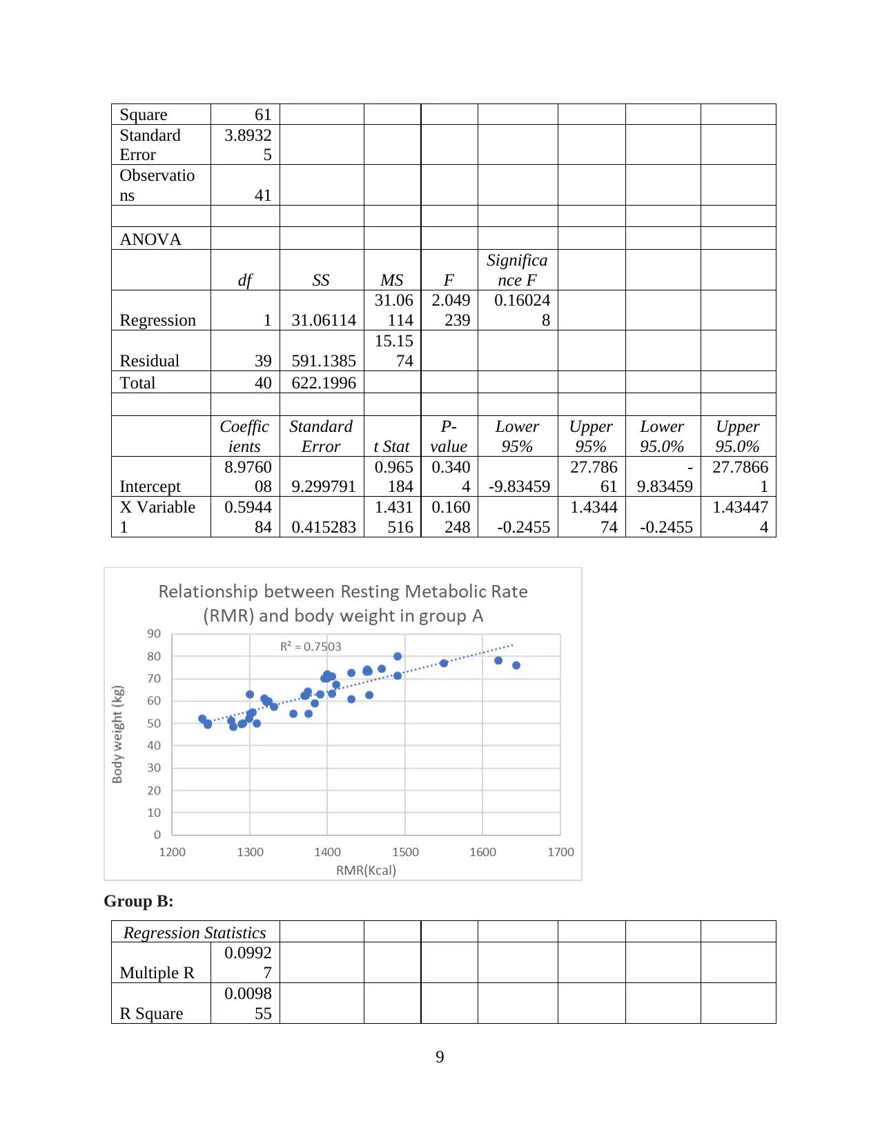
Group B:
Regression Statistics
Multiple R
0.0992
7
R Square
0.0098
55
9
Standard
Error
3.8932
5
Observatio
ns 41
ANOVA
df SS MS F
Significa
nce F
Regression 1 31.06114
31.06
114
2.049
239
0.16024
8
Residual 39 591.1385
15.15
74
Total 40 622.1996
Coeffic
ients
Standard
Error t Stat
P-
value
Lower
95%
Upper
95%
Lower
95.0%
Upper
95.0%
Intercept
8.9760
08 9.299791
0.965
184
0.340
4 -9.83459
27.786
61
-
9.83459
27.7866
1
X Variable
1
0.5944
84 0.415283
1.431
516
0.160
248 -0.2455
1.4344
74 -0.2455
1.43447
4
Group B:
Regression Statistics
Multiple R
0.0992
7
R Square
0.0098
55
9
⊘ This is a preview!⊘
Do you want full access?
Subscribe today to unlock all pages.
Trusted by 1+ million students worldwide
Adjusted R
Square
-
0.0155
3
Standard
Error
6.2573
86
Observatio
ns 41
ANOVA
df SS MS F
Significa
nce F
Regression 1 15.19815
15.19
815
0.388
155
0.53689
7
Residual 39 1527.04
39.15
487
Total 40 1542.238
Coeffic
ients
Standard
Error t Stat
P-
value
Lower
95%
Upper
95%
Lower
95.0%
Upper
95.0%
Intercept
39.358
39 7.086608
5.553
911
2.16E
-06
25.0243
8
53.692
41
25.0243
8
53.6924
1
X Variable
1
-
0.1253
3 0.201158
-
0.623
02
0.536
897 -0.53221
0.2815
55
-
0.53221
0.28155
5
10
Paraphrase This Document
Need a fresh take? Get an instant paraphrase of this document with our AI Paraphraser
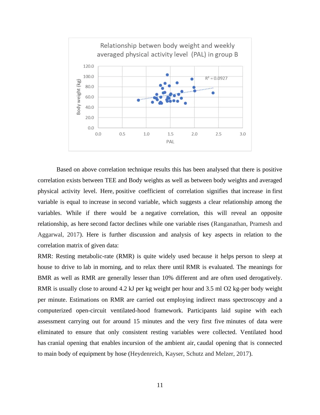
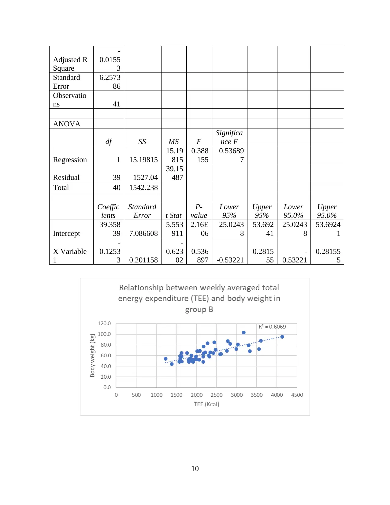
Based on above correlation technique results this has been analysed that there is positive
correlation exists between TEE and Body weights as well as between body weights and averaged
physical activity level. Here, positive coefficient of correlation signifies that increase in first
variable is equal to increase in second variable, which suggests a clear relationship among the
variables. While if there would be a negative correlation, this will reveal an opposite
relationship, as here second factor declines while one variable rises (Ranganathan, Pramesh and
Aggarwal, 2017). Here is further discussion and analysis of key aspects in relation to the
correlation matrix of given data:
RMR: Resting metabolic-rate (RMR) is quite widely used because it helps person to sleep at
house to drive to lab in morning, and to relax there until RMR is evaluated. The meanings for
BMR as well as RMR are generally lesser than 10% different and are often used derogatively.
RMR is usually close to around 4.2 kJ per kg weight per hour and 3.5 ml O2 kg-per body weight
per minute. Estimations on RMR are carried out employing indirect mass spectroscopy and a
computerized open-circuit ventilated-hood framework. Participants laid supine with each
assessment carrying out for around 15 minutes and the very first five minutes of data were
eliminated to ensure that only consistent resting variables were collected. Ventilated hood
has cranial opening that enables incursion of the ambient air, caudal opening that is connected
to main body of equipment by hose (Heydenreich, Kayser, Schutz and Melzer, 2017).
11
Metabolic equivalents (MET): One MET being equal to the amount of oxygen intake (V to O2)
at rests or in quiet sitting posture and is comparable to 3.5 ml/min/kg of body mass or 1
kcal/hour/kg body mass. The MET of given activity is ratio of metabolic rate of an activity
to resting metabolic rate which indicates how often times the energy consumption of given
activity is greater than that of energy expenditure at idle (Zusman and et.al., 2019).
Conclusion
From above study-report, this has been articulated that scientific report provides
comprehensive details regarding each aspect of data selected. The study helps researchers and
analysts to thoroughly analyse each and every variable as well as to assess the key relation
among different variables. Throughout the Vigorous Exercise Collection, detailed MET
calculations and thus EE estimates are developed for different sports exercise, with roles ranging
from 0.9 MET (going to sleep) to 18 MET (sleeping). Due to differences in body weight,
dyslipidemia, age and gender, real electricity prices can differ between individuals. METs are
defined as EE levels per kg of body weight to account for differences in body mass. Usage of
physical activities Compilation enables the measurement of daily EAs by journals of physical
activity, providing information on the nature, magnitude and period of each exercise used for the
traditional life. A full collection of electricity prices will be sent to Moodle for the different
exercise exercises.
12
⊘ This is a preview!⊘
Do you want full access?
Subscribe today to unlock all pages.
Trusted by 1+ million students worldwide
1 out of 18
Related Documents


Your All-in-One AI-Powered Toolkit for Academic Success.
+13062052269
info@desklib.com
Available 24*7 on WhatsApp / Email
![[object Object]](/_next/static/media/star-bottom.7253800d.svg)
Unlock your academic potential
Copyright © 2020–2026 A2Z Services. All Rights Reserved. Developed and managed by ZUCOL.