Project Proposal: Modeling Influenza Spread and Vaccine Effectiveness

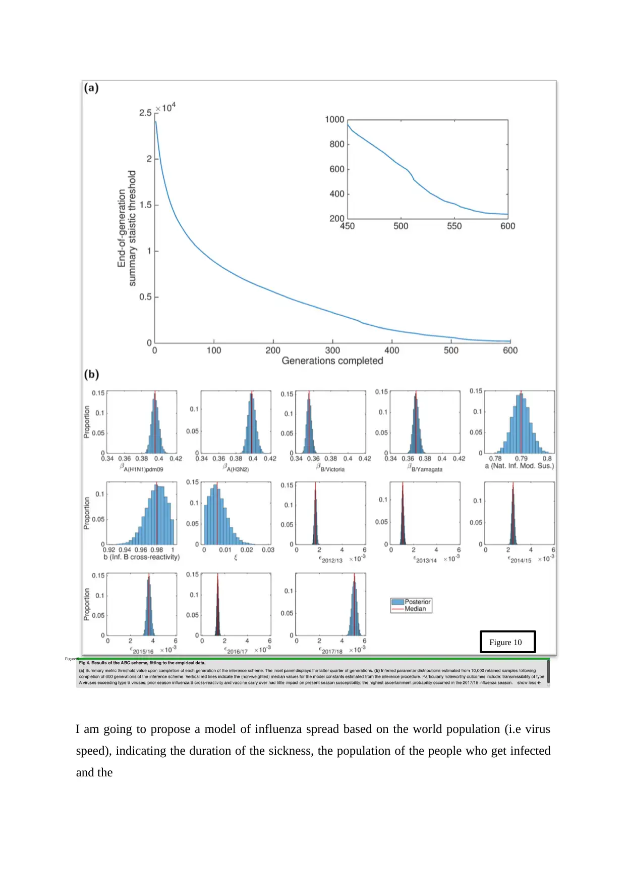
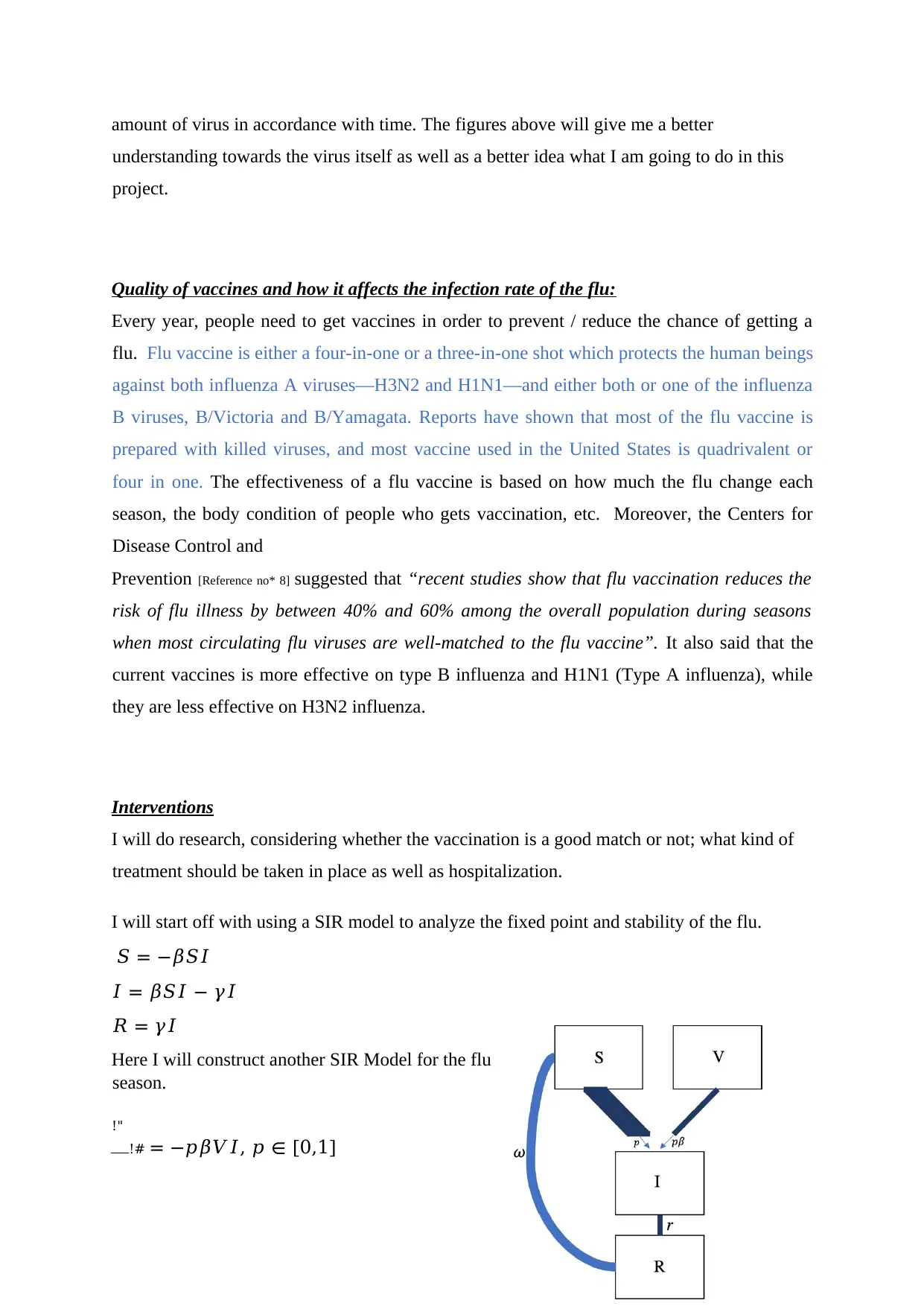
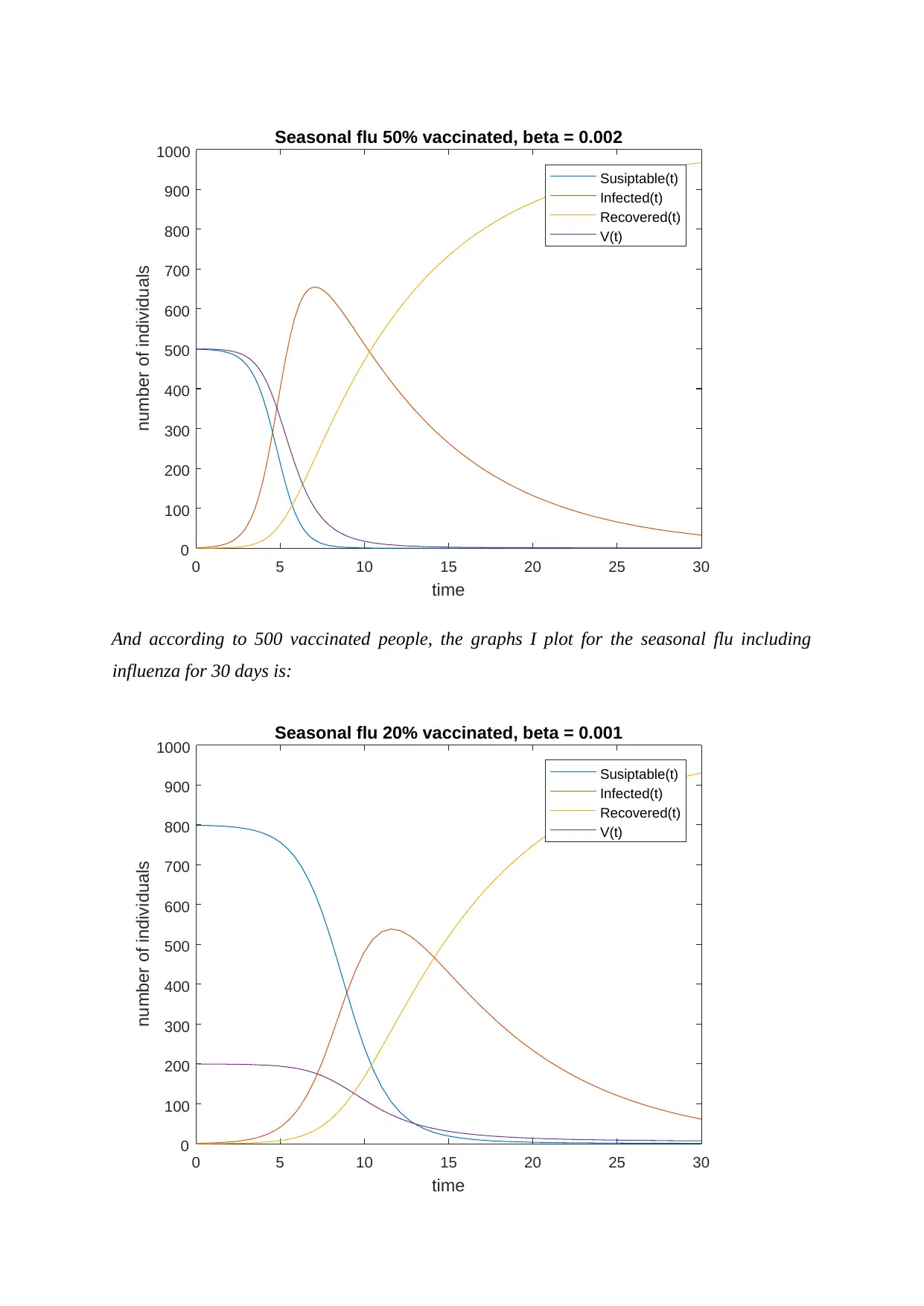
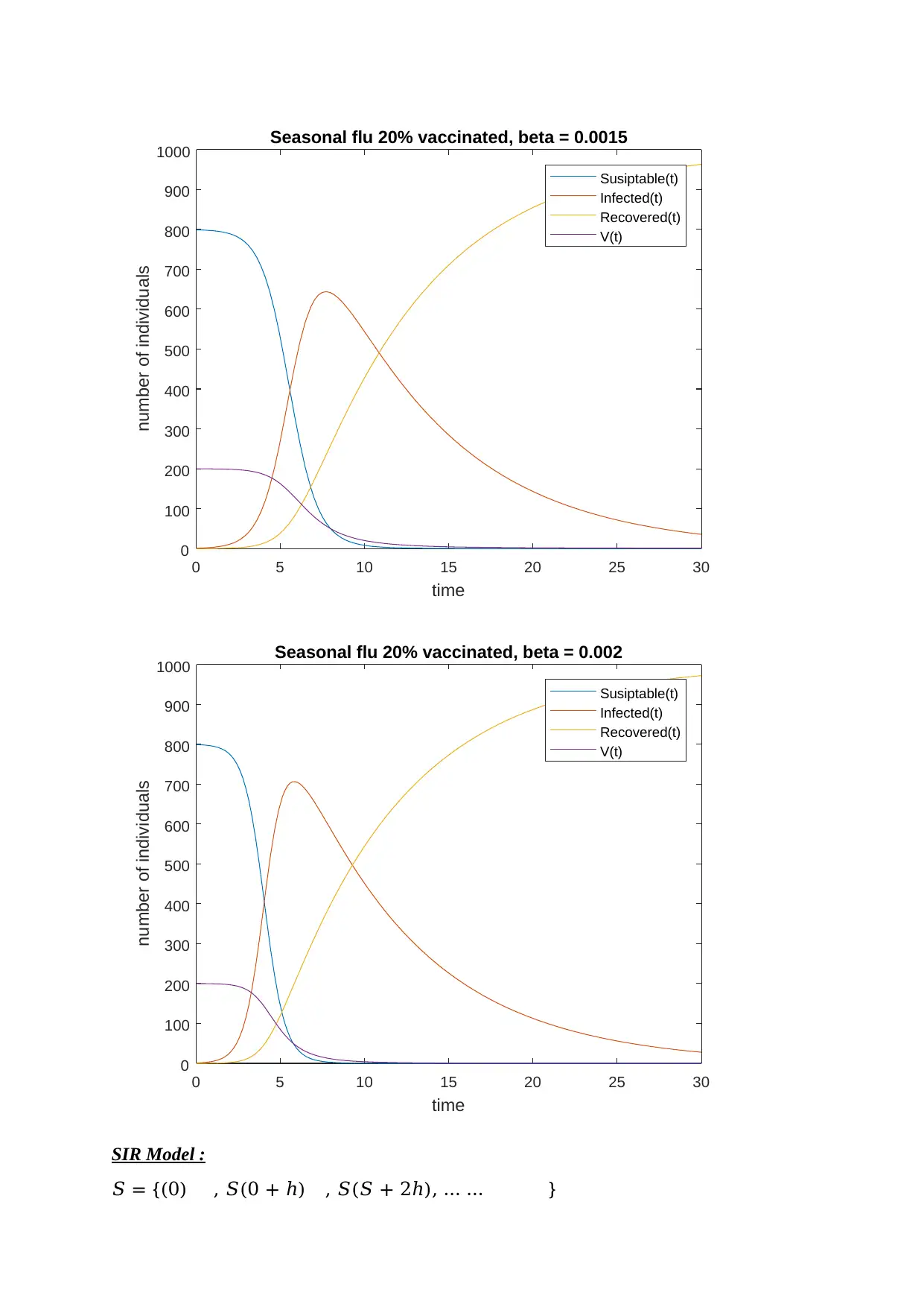
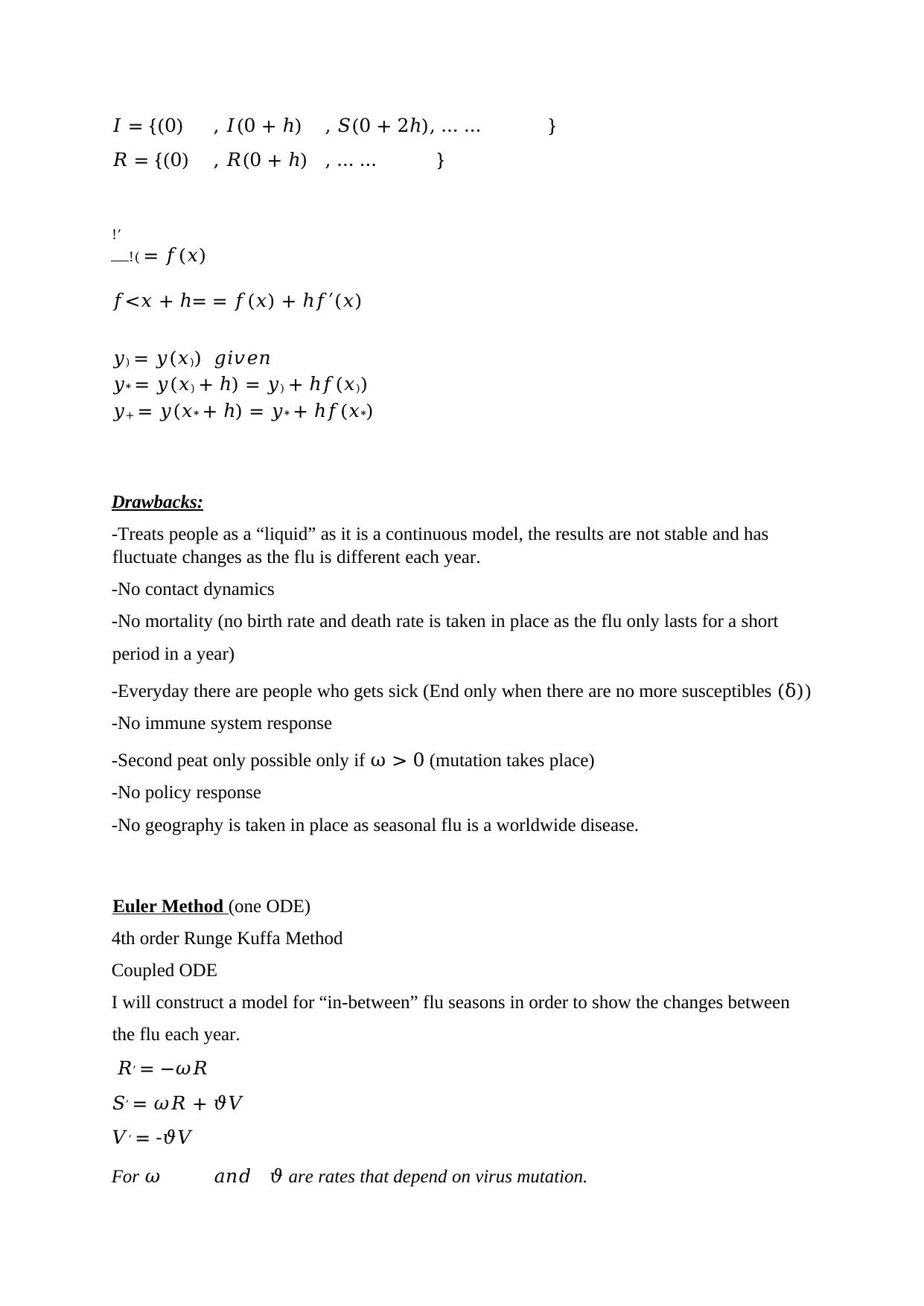
This project proposal outlines a model for analyzing the spread of influenza, focusing on seasonal flu dynamics, vaccination effectiveness, and potential treatment interventions. The project will utilize SIR models to simulate the infection rate, recovery rate, and the impact of vaccination on the population. The proposal includes an introduction to influenza, its transmission, and the need for new drugs and vaccines. The project will model the flu spread based on world population, sickness duration, infection rates, and virus quantity over time. The student proposes to use existing figures from research papers to provide a better understanding of the virus and guide the modeling process. The analysis will include examining the effectiveness of vaccines, different treatment options, and hospitalization rates. The proposal includes two SIR models, one for regular flu seasons and another for in-between seasons, considering mutation rates. The student will use MATLAB code to simulate the models and analyze the results, discussing the drawbacks of the model, such as the continuous nature of the model and the absence of contact dynamics. The project also includes a comprehensive bibliography and MATLAB code for simulations.

Project Proposal
Scarlett, Qing Sun
#215320302
Introduction
Influenza, also known as flu, is a respiratory infectious disease, as well as a global threat to
humans due to the fact it can be transmitted by having direct contact with infected people and
the contaminated objects, as well as the droplets in the air (i.e people’s cough and sneeze).
The Centers for Disease Control and Prevention has pointed out that people infected with
influenza can transmit the pathogen to others up to about 6 feet away2. Nevertheless, after the
virus enters human body, it normally takes 2-4 days for the symptoms to begin1. It also stated
that "you may be able to pass on the flu to someone else before you know you are sick, as
well as while you are sick. Some people may not show any symptoms after being infected by
a flu virus.
During this time, those people may still spread the virus to others."
According to the article “A Roadmap for Influenza Research”, published by Viktor Müller,
“the influenza viruses are characterized by segmented, negative-strand RNA genomes
requiring an RNA-dependent RNA polymerase of viral origin for replication. The particular
structure of the influenza virus genome and function of its viral proteins enable antigenic drift
and antigenic shift.’ Very small changes based on the genetic makeup of the influenza strains
have been found to be referred as antigenic drift. However, when a flu strain mutates to a very
high extent, major changes occurs in the antigenic determinants which results in an antigenic
shift.
Moreover, studies and statistics have suggested that flu are constantly changing every
different each year. This is the reason why doctors and experimental scientists need to
develop new drugs, vaccines and adjuvant to help us prevent from getting infected. An article
has suggested that there are between 291,000 and 646,000 people worldwide are being killed
by flu each year.
Modelling:

figure 1 modelling from “A Roadmap for Influenza Research”
figure 2 modelling from “A Roadmap for Influenza Research”

Figure 3 from “Modeling influenza epidemics and pandemics”
Figure 4 from "Viral Kinetic Modeling: State of the Art"

Figure 5 from "Influenza interaction with co-circulating pathogens and its impact on
surveillance, pathogenesis, and epidemic profile"

The 4 figures (6,7,8 and 9 I labeled) above , from "Mathematical Analysis of Influenza A
Dynamics in the Emergence of Drug Resistance" indicates how drug resistance can affect
people who got infected by flu.
Figure 6 Figure 7
Figure 8 Figure 9

I am going to propose a model of influenza spread based on the world population (i.e virus
speed), indicating the duration of the sickness, the population of the people who get infected
and the
Figure 10
Figure 9

amount of virus in accordance with time. The figures above will give me a better
understanding towards the virus itself as well as a better idea what I am going to do in this
project.
Quality of vaccines and how it affects the infection rate of the flu:
Every year, people need to get vaccines in order to prevent / reduce the chance of getting a
flu. Flu vaccine is either a four-in-one or a three-in-one shot which protects the human beings
against both influenza A viruses—H3N2 and H1N1—and either both or one of the influenza
B viruses, B/Victoria and B/Yamagata. Reports have shown that most of the flu vaccine is
prepared with killed viruses, and most vaccine used in the United States is quadrivalent or
four in one. The effectiveness of a flu vaccine is based on how much the flu change each
season, the body condition of people who gets vaccination, etc. Moreover, the Centers for
Disease Control and
Prevention [Reference no* 8] suggested that “recent studies show that flu vaccination reduces the
risk of flu illness by between 40% and 60% among the overall population during seasons
when most circulating flu viruses are well-matched to the flu vaccine”. It also said that the
current vaccines is more effective on type B influenza and H1N1 (Type A influenza), while
they are less effective on H3N2 influenza.
Interventions
I will do research, considering whether the vaccination is a good match or not; what kind of
treatment should be taken in place as well as hospitalization.
I will start off with using a SIR model to analyze the fixed point and stability of the flu.
𝑆 = −𝛽𝑆𝐼
𝐼 = 𝛽𝑆𝐼 − 𝛾𝐼
𝑅 = 𝛾𝐼
Here I will construct another SIR Model for the flu
season.
!"
!# = −𝑝𝛽𝑉𝐼, 𝑝 ∈ [0,1]

!$
!# = −𝛽𝑆𝐼 + 𝜔𝑅
!%
! # = 𝛽𝑆𝐼 − 𝛾𝐼 + 𝑝𝛽𝑉𝐼
!&
!# = 𝛾𝐼 − 𝜔𝑅
According to the national report the regular interaction of an infected person with the
population is 5% or 5 person for per 100 population. On the other hand, the average
infection rate of seasonal flue is 3%. The lower limit is 2% and the upper limit is 4%.
Therefore, the overall infection rate in normal seasons 𝛽1= 0.05x0.03=0.0015;
𝛽2=0.001; and 𝛽3=0.002
As discussed earlier the recovery rate of seasonal flue depends on
the population who is not under the influenza infected population.
Influenza has zero recovery rate without treatment. However, only
30% among the seasonal flue population suffer from influenza.
Hence, 70% is common cold flue. At the same time, in case of
seasonal flue only 5 days are required to recovery or in 0.2 recovery
ratio per day. Therefore the recovery rate of infected peoples
𝛾=(0.7x0.2)=0.14
Recent studies show that flu vaccination reduces the risk of flu
illness by between 40% and 60% among the overall population
during seasons when most circulating flu viruses are well-matched to
the flu vaccine. Therefore the average effective vaccination is 50%.
Hence, rate of reinvented from vaccination is 0.5
The base vaccinated population can ranged from 20% to 50%.
Therefore, in 1000 population the base vaccinated population can be
200 or 500.
And according to 500 vaccinated people, the graphs I plot for the seasonal flu including
influenza for 30 days is:

0 5 10 15 20 25 30
time
0
100
200
300
400
500
600
700
800
900
number of individuals
Seasonal flu 50% vaccinated, beta = 0.001
Susiptable(t)
Infected(t)
Recovered(t)
V(t)
0 5 10 15 20 25 30
time
0
100
200
300
400
500
600
700
800
900
1000
number of individuals
Seasonal flu 50% vaccinated, beta = 0.0015
Susiptable(t)
Infected(t)
Recovered(t)
V(t)

0 5 10 15 20 25 30
time
0
100
200
300
400
500
600
700
800
900
1000
number of individuals
Seasonal flu 50% vaccinated, beta = 0.002
Susiptable(t)
Infected(t)
Recovered(t)
V(t)
And according to 500 vaccinated people, the graphs I plot for the seasonal flu including
influenza for 30 days is:
0 5 10 15 20 25 30
time
0
100
200
300
400
500
600
700
800
900
1000
number of individuals
Seasonal flu 20% vaccinated, beta = 0.001
Susiptable(t)
Infected(t)
Recovered(t)
V(t)

0 5 10 15 20 25 30
time
0
100
200
300
400
500
600
700
800
900
1000
number of individuals
Seasonal flu 20% vaccinated, beta = 0.0015
Susiptable(t)
Infected(t)
Recovered(t)
V(t)
0 5 10 15 20 25 30
time
0
100
200
300
400
500
600
700
800
900
1000
number of individuals
Seasonal flu 20% vaccinated, beta = 0.002
Susiptable(t)
Infected(t)
Recovered(t)
V(t)
SIR Model :
𝑆 = {(0) , 𝑆(0 + ℎ) , 𝑆(𝑆 + 2ℎ), … … }

𝐼 = {(0) , 𝐼(0 + ℎ) , 𝑆(0 + 2ℎ), … … }
𝑅 = {(0) , 𝑅(0 + ℎ) , … … }
!’
!( = 𝑓(𝑥)
𝑓<𝑥 + ℎ= = 𝑓(𝑥) + ℎ𝑓′(𝑥)
𝑦) = 𝑦(𝑥)) 𝑔𝑖𝑣𝑒𝑛
𝑦* = 𝑦(𝑥) + ℎ) = 𝑦) + ℎ𝑓(𝑥))
𝑦+ = 𝑦(𝑥* + ℎ) = 𝑦* + ℎ𝑓(𝑥*)
Drawbacks:
-Treats people as a “liquid” as it is a continuous model, the results are not stable and has
fluctuate changes as the flu is different each year.
-No contact dynamics
-No mortality (no birth rate and death rate is taken in place as the flu only lasts for a short
period in a year)
-Everyday there are people who gets sick (End only when there are no more susceptibles (δ))
-No immune system response
-Second peat only possible only if ω > 0 (mutation takes place)
-No policy response
-No geography is taken in place as seasonal flu is a worldwide disease.
Euler Method (one ODE)
4th order Runge Kuffa Method
Coupled ODE
I will construct a model for “in-between” flu seasons in order to show the changes between
the flu each year.
𝑅, = −𝜔𝑅
𝑆, = 𝜔𝑅 + 𝜗𝑉
𝑉, = -𝜗𝑉
For 𝜔 𝑎𝑛𝑑 𝜗 are rates that depend on virus mutation.

From the above researches and evidences because of the the mutation rate of the virus that
causes the reoccurrence of seasonal flue in recovered population is 0.03 and the vaccinated
population 0.02. Hence for two different vaccinated percentage 20%, 30% and 50% the, in-
between seasonal flue SIR model will be:
0 5 10 15 20 25 30
time
0
100
200
300
400
500
600
700
800
900
number of individuals
Seasonal inbetween flu and 20% vaccinated
Susiptable(t)
Infected(t)
Recovered(t)
V(t)

0 5 10 15 20 25 30
time
0
100
200
300
400
500
600
700
800
number of individuals
Seasonal inbetween flu and 30% vaccinated
Susiptable(t)
Infected(t)
Recovered(t)
V(t)
0 5 10 15 20 25 30
time
0
100
200
300
400
500
600
700
800
number of individuals
Seasonal inbetween flu and 50% vaccinated
Susiptable(t)
Infected(t)
Recovered(t)
V(t)

Bibliography:
1. Modeling Influenza Virus Infection: A Roadmap for Influenza Research
https://www.ncbi.nlm.nih.gov/pmc/articles/PMC4632383/
2. Modeling influenza epidemics and pandemics: insights into the future of swine
flu (H1N1)
https://www.ncbi.nlm.nih.gov/pmc/articles/PMC2715422/
3. How Flu Spreads https://www.cdc.gov/flu/about/disease/spread.htm
4. Viral Kinetic Modeling: State of the Art
https://www.researchgate.net/figure/Mathematical-modeling-of-influenza-kinetics-
aSchematic-of-the-model-for-influenza_fig4_263397901
5. Influenza interaction with co-circulating pathogens and its impact on
surveillance, pathogenesis, and epidemic profile: A key role for mathematical
modelling
https://journals.plos.org/plospathogens/article?id=10.1371/journal.ppat.1006770
6. Mathematical Analysis of Influenza A Dynamics in the Emergence of Drug
Resistance
https://www.hindawi.com/journals/cmmm/2018/2434560/
7. Flu Vaccine Selections Suggest This Year’s Shot May Be Off the Mark
https://www.scientificamerican.com/article/flu-vaccine-selections-suggest-this-
yearsshot-may-be-off-the-mark/
8. Vaccine Effectiveness: How Well Do the Flu Vaccines Work?

https://www.cdc.gov/flu/vaccines-work/vaccineeffect.htm
Appendix: Code (Matlab)
function start
%-------------------------------------------------------------------------
% User Section 1: Definition of model parameters
%-------------------------------------------------------------------------
param.beta = 0.0015; % parameter 'beta' of the model (5/100)*(3/100)
param.gama = 0.14; %parameter 'gama' of the model(1/5)*(70/100)
param.p = 0.5; %parameter 'p' of the model
% This is the title string for the plot window.
model_title = 'Seasonal flu 20% vaccinated, beta = 0.0015';
%-------------------------------------------------------------------------
% User Section 2: Definition of initial conditions
%-------------------------------------------------------------------------
initial.S = 799; % set the initial value of 'S'
initial.I = 1; % the initial value of 'I'
initial.R = 0; % the initial value of 'R'
initial.V = 200; % the initial value of 'V'
%-------------------------------------------------------------------------
% User Section 3: Definition of the simulation time
%-------------------------------------------------------------------------
end_time = 30;
%-------------------------------------------------------------------------
% User Section 4: Definition of the ODE system
%-------------------------------------------------------------------------
function deriv = ode_system (t, x, param)
% Function to calculate derivatives of the SIR model
%
% Input:
% t: Time (not used in this example because there is no explicit
% time dependence).
% x: Vector of the current values of all variables in the same
% order as you defined the inital values: S, I, R
% param: Used to pass parameter values.
% Output:
% deriv: Column vector of derivatives, must be the same order as the
% input vector x.
S = x(1);
I = x(2);
R = x(3);
V = x(4);
dS = -param.beta * S * I;
dI = +(param.beta * S * I) + (param.beta * param.p * V * I) - (param.gama *
I);
% Note: because S+I+R=constant, this equation could actually be omitted,
% and R at any time point could simply be calculated as N-S-I.
dR = param.gama * I;
dV = -param.beta * param.p * V * I;
deriv = [dS; dI; dR; dV];
end
%-------------------------------------------------------------------------

% Now we solve the ODE system and plot the results
%-------------------------------------------------------------------------
% Calculate and print R_0 on the screen
N = initial.S + initial.R + initial.I + initial.V;
% Extract initial values from the 'initial' structure and collect them
% in a column vector for use in 'ode45'.
initial_values = [];
variable_names = fieldnames(initial);
for i=1:length(variable_names)
initial_values = [initial_values; initial.(variable_names{i})];
end
% integrate the ODE system
[t, y] = ode45(@(t, x) ode_system(t, x, param), ...
[0 end_time], ...
initial_values, ...
[]);
% plot the results
plot(t, y);
legend('Susiptable(t)','Infected(t)','Recovered(t)','V(t)');
xlabel('time');
ylabel('number of individuals');
title(model_title);
end
function start
%-------------------------------------------------------------------------
% User Section 1: Definition of model parameters
%-------------------------------------------------------------------------
param.beta = 0.001; % parameter 'beta' of the model (5/100)*(3/100)
param.gama = 0.14; %parameter 'gama' of the model(1/5)*(70/100)
param.p = 0.5; %parameter 'p' of the model
% This is the title string for the plot window.
model_title = 'Seasonal flu 50% vaccinated, beta = 0.001';
%-------------------------------------------------------------------------
% User Section 2: Definition of initial conditions
%-------------------------------------------------------------------------
initial.S = 499; % set the initial value of 'S'
initial.I = 1; % the initial value of 'I'
initial.R = 0; % the initial value of 'R'
initial.V = 500; % the initial value of 'V'
%-------------------------------------------------------------------------
% User Section 3: Definition of the simulation time
%-------------------------------------------------------------------------
end_time = 30;
%-------------------------------------------------------------------------
% User Section 4: Definition of the ODE system
%-------------------------------------------------------------------------
function deriv = ode_system (t, x, param)
% Function to calculate derivatives of the SIR model
%
% Input:
% t: Time (not used in this example because there is no explicit

% time dependence).
% x: Vector of the current values of all variables in the same
% order as you defined the inital values: S, I, R
% param: Used to pass parameter values.
% Output:
% deriv: Column vector of derivatives, must be the same order as the
% input vector x.
S = x(1);
I = x(2);
R = x(3);
V = x(4);
dS = -param.beta * S * I;
dI = +(param.beta * S * I) + (param.beta * param.p * V * I) - (param.gama *
I);
% Note: because S+I+R=constant, this equation could actually be omitted,
% and R at any time point could simply be calculated as N-S-I.
dR = param.gama * I;
dV = -param.beta * param.p * V * I;
deriv = [dS; dI; dR; dV];
end
%-------------------------------------------------------------------------
% Now we solve the ODE system and plot the results
%-------------------------------------------------------------------------
% Calculate and print R_0 on the screen
N = initial.S + initial.R + initial.I + initial.V;
% Extract initial values from the 'initial' structure and collect them
% in a column vector for use in 'ode45'.
initial_values = [];
variable_names = fieldnames(initial);
for i=1:length(variable_names)
initial_values = [initial_values; initial.(variable_names{i})];
end
% integrate the ODE system
[t, y] = ode45(@(t, x) ode_system(t, x, param), ...
[0 end_time], ...
initial_values, ...
[]);
% plot the results
plot(t, y);
legend('Susiptable(t)','Infected(t)','Recovered(t)','V(t)');
xlabel('time');
ylabel('number of individuals');
title(model_title);
end
function start
%-------------------------------------------------------------------------
% User Section 1: Definition of model parameters
%-------------------------------------------------------------------------

param.beta = 0.002; % parameter 'beta' of the model (5/100)*(3/100)
param.gama = 0.14; %parameter 'gama' of the model(1/5)*(70/100)
param.p = 0.5; %parameter 'p' of the model
% This is the title string for the plot window.
model_title = 'Seasonal flu 50% vaccinated, beta = 0.002';
%-------------------------------------------------------------------------
% User Section 2: Definition of initial conditions
%-------------------------------------------------------------------------
initial.S = 499; % set the initial value of 'S'
initial.I = 1; % the initial value of 'I'
initial.R = 0; % the initial value of 'R'
initial.V = 500; % the initial value of 'V'
%-------------------------------------------------------------------------
% User Section 3: Definition of the simulation time
%-------------------------------------------------------------------------
end_time = 30;
%-------------------------------------------------------------------------
% User Section 4: Definition of the ODE system
%-------------------------------------------------------------------------
function deriv = ode_system (t, x, param)
% Function to calculate derivatives of the SIR model
%
% Input:
% t: Time (not used in this example because there is no explicit
% time dependence).
% x: Vector of the current values of all variables in the same
% order as you defined the inital values: S, I, R
% param: Used to pass parameter values.
% Output:
% deriv: Column vector of derivatives, must be the same order as the
% input vector x.
S = x(1);
I = x(2);
R = x(3);
V = x(4);
dS = -param.beta * S * I;
dI = +(param.beta * S * I) + (param.beta * param.p * V * I) - (param.gama *
I);
% Note: because S+I+R=constant, this equation could actually be omitted,
% and R at any time point could simply be calculated as N-S-I.
dR = param.gama * I;
dV = -param.beta * param.p * V * I;
deriv = [dS; dI; dR; dV];
end
%-------------------------------------------------------------------------
% Now we solve the ODE system and plot the results
%-------------------------------------------------------------------------
% Calculate and print R_0 on the screen
N = initial.S + initial.R + initial.I + initial.V;
% Extract initial values from the 'initial' structure and collect them
% in a column vector for use in 'ode45'.
initial_values = [];
variable_names = fieldnames(initial);
for i=1:length(variable_names)
initial_values = [initial_values; initial.(variable_names{i})];
end

% integrate the ODE system
[t, y] = ode45(@(t, x) ode_system(t, x, param), ...
[0 end_time], ...
initial_values, ...
[]);
% plot the results
plot(t, y);
legend('Susiptable(t)','Infected(t)','Recovered(t)','V(t)');
xlabel('time');
ylabel('number of individuals');
title(model_title);
end
Appendix: In-between Seasons
function start
%-------------------------------------------------------------------------
% User Section 1: Definition of model parameters
%-------------------------------------------------------------------------
param.beta = 0.0015; % parameter 'beta' of the model (5/100)*(3/100)
param.gama = 0.14; %parameter 'gama' of the model(1/5)*(70/100)
param.p = 0.5; %parameter 'p' of the model
param.omega = 0.03;
param.upsilon=0.02;
% This is the title string for the plot window.
model_title = 'Seasonal inbetween flu and 20% vaccinated';
%-------------------------------------------------------------------------
% User Section 2: Definition of initial conditions
%-------------------------------------------------------------------------
initial.S = 799; % set the initial value of 'S'
initial.I = 1; % the initial value of 'I'
initial.R = 0; % the initial value of 'R'
initial.V = 200; % the initial value of 'V'
%-------------------------------------------------------------------------
% User Section 3: Definition of the simulation time
%-------------------------------------------------------------------------
end_time = 30;
%-------------------------------------------------------------------------
% User Section 4: Definition of the ODE system
%-------------------------------------------------------------------------
function deriv = ode_system (t, x, param)
% Function to calculate derivatives of the SIR model
% t: Time (not used in this example because there is no explicit
% time dependence).
% x: Vector of the current values of all variables in the same
% order as you defined the inital values: S, I, R, V
% param: Used to pass parameter values.

S = x(1);
I = x(2);
R = x(3);
V = x(4);
dS = -(param.beta * S * I)+(param.omega * R)+(param.upsilon * V);
dI = +(param.beta * S * I) + (param.beta * param.p* V * I) - (param.gama *
I);
% Note: because S+I+R=constant, this equation could actually be omitted,
% and R at any time point could simply be calculated as N-S-I.
dR = +(param.gama * I) - (param.omega * R);
dV = -(param.beta * param.p* V * I) - (param.upsilon * V);
deriv = [dS; dI; dR; dV];
end
%-------------------------------------------------------------------------
% Now we solve the ODE system and plot the results
%-------------------------------------------------------------------------
% Calculate and print R_0 on the screen
N = initial.S + initial.R + initial.I + initial.V;
% Extract initial values from the 'initial' structure and collect them
% in a column vector for use in 'ode45'.
initial_values = [];
variable_names = fieldnames(initial);
for i=1:length(variable_names)
initial_values = [initial_values; initial.(variable_names{i})];
end
% integrate the ODE system
[t, y] = ode45(@(t, x) ode_system(t, x, param), ...
[0 end_time], ...
initial_values, ...
[]);
% plot the results
plot(t, y);
legend('Susiptable(t)','Infected(t)','Recovered(t)','V(t)');
xlabel('time');
ylabel('number of individuals');
title(model_title);
end
function start
%-------------------------------------------------------------------------
% User Section 1: Definition of model parameters
%-------------------------------------------------------------------------
param.beta = 0.0015; % parameter 'beta' of the model (5/100)*(3/100)
param.gama = 0.14; %parameter 'gama' of the model(1/5)*(70/100)
param.p = 0.5; %parameter 'p' of the model
param.omega = 0.03;
param.upsilon=0.02;
% This is the title string for the plot window.
model_title = 'Seasonal inbetween flu and 500% vaccinated';

%-------------------------------------------------------------------------
% User Section 2: Definition of initial conditions
%-------------------------------------------------------------------------
initial.S = 499; % set the initial value of 'S'
initial.I = 1; % the initial value of 'I'
initial.R = 0; % the initial value of 'R'
initial.V = 500; % the initial value of 'V'
%-------------------------------------------------------------------------
% User Section 3: Definition of the simulation time
%-------------------------------------------------------------------------
end_time = 30;
%-------------------------------------------------------------------------
% User Section 4: Definition of the ODE system
%-------------------------------------------------------------------------
function deriv = ode_system (t, x, param)
% Function to calculate derivatives of the SIR model
% t: Time (not used in this example because there is no explicit
% time dependence).
% x: Vector of the current values of all variables in the same
% order as you defined the inital values: S, I, R, V
% param: Used to pass parameter values.
S = x(1);
I = x(2);
R = x(3);
V = x(4);
dS = -(param.beta * S * I)+(param.omega * R)+(param.upsilon * V);
dI = +(param.beta * S * I) + (param.beta * param.p* V * I) - (param.gama *
I);
% Note: because S+I+R=constant, this equation could actually be omitted,
% and R at any time point could simply be calculated as N-S-I.
dR = +(param.gama * I) - (param.omega * R);
dV = -(param.beta * param.p* V * I) - (param.upsilon * V);
deriv = [dS; dI; dR; dV];
end
%-------------------------------------------------------------------------
% Now we solve the ODE system and plot the results
%-------------------------------------------------------------------------
% Calculate and print R_0 on the screen
N = initial.S + initial.R + initial.I + initial.V;
% Extract initial values from the 'initial' structure and collect them
% in a column vector for use in 'ode45'.
initial_values = [];
variable_names = fieldnames(initial);
for i=1:length(variable_names)
initial_values = [initial_values; initial.(variable_names{i})];
end
% integrate the ODE system
[t, y] = ode45(@(t, x) ode_system(t, x, param), ...
[0 end_time], ...
initial_values, ...
[]);

% plot the results
plot(t, y);
legend('Susiptable(t)','Infected(t)','Recovered(t)','V(t)');
xlabel('time');
ylabel('number of individuals');
title(model_title);
end