University Electrical Engineering: Sensors and Measurement Assignment

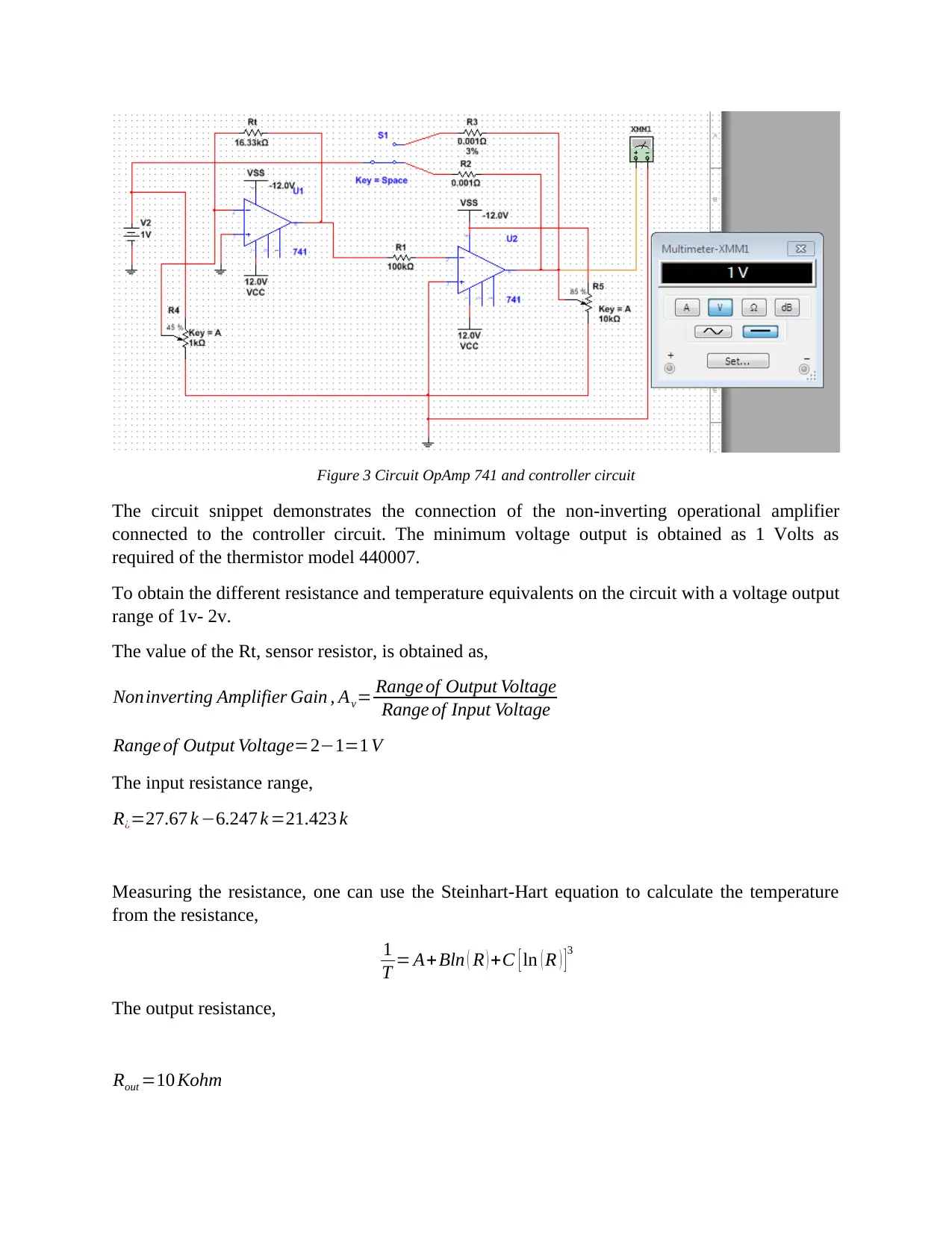
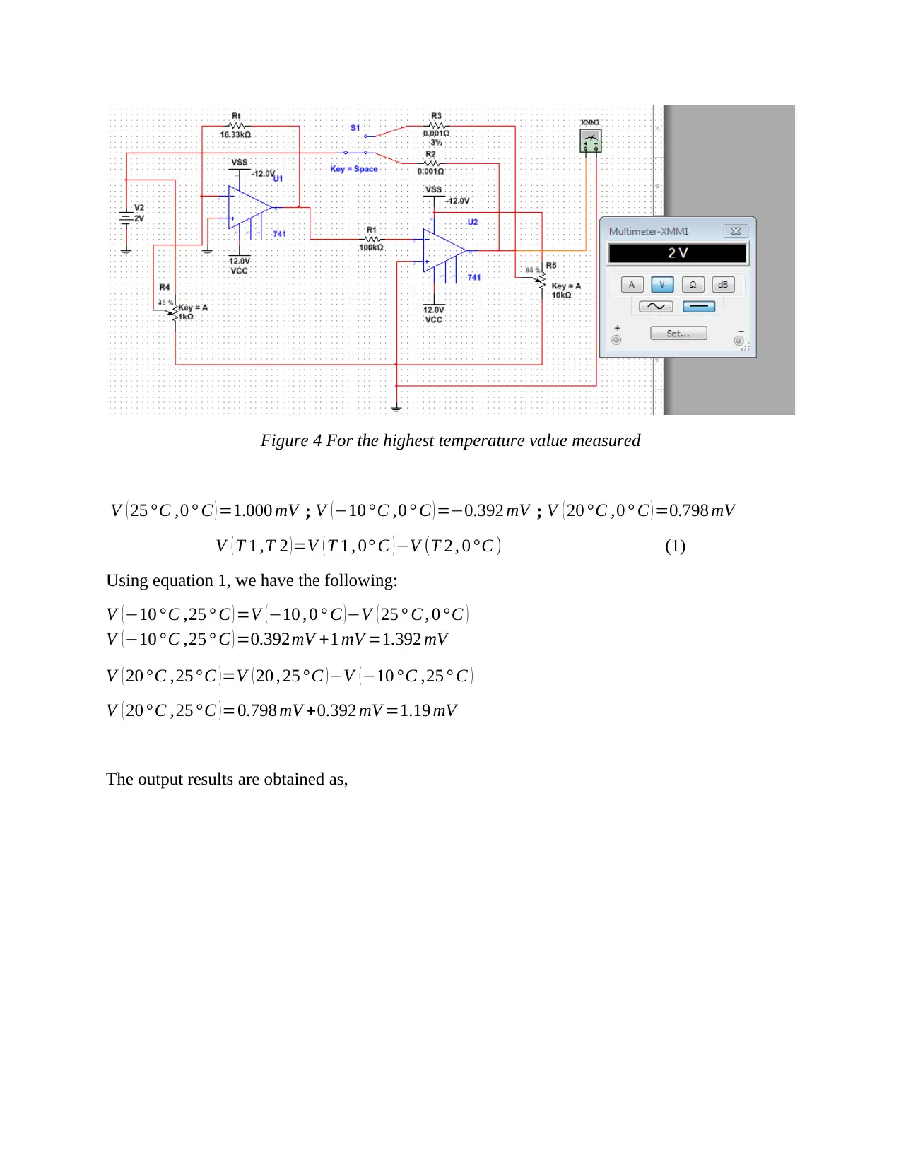
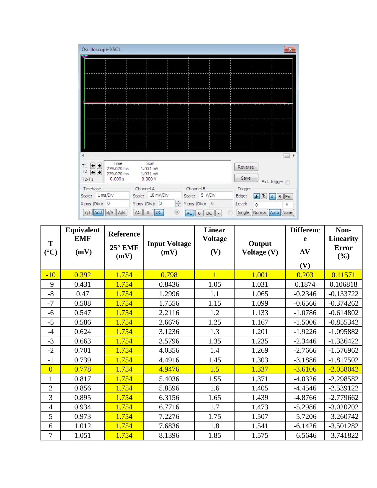
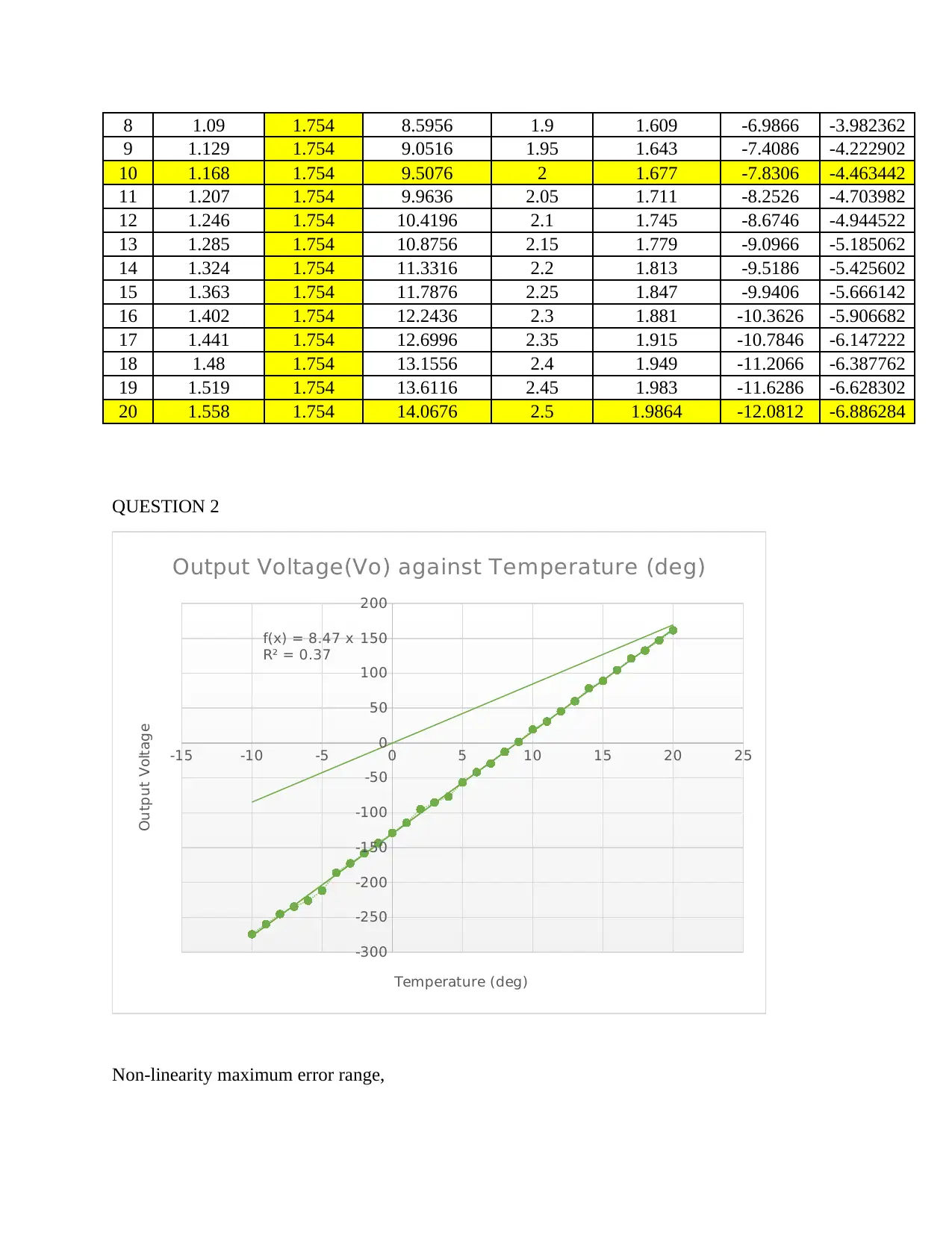
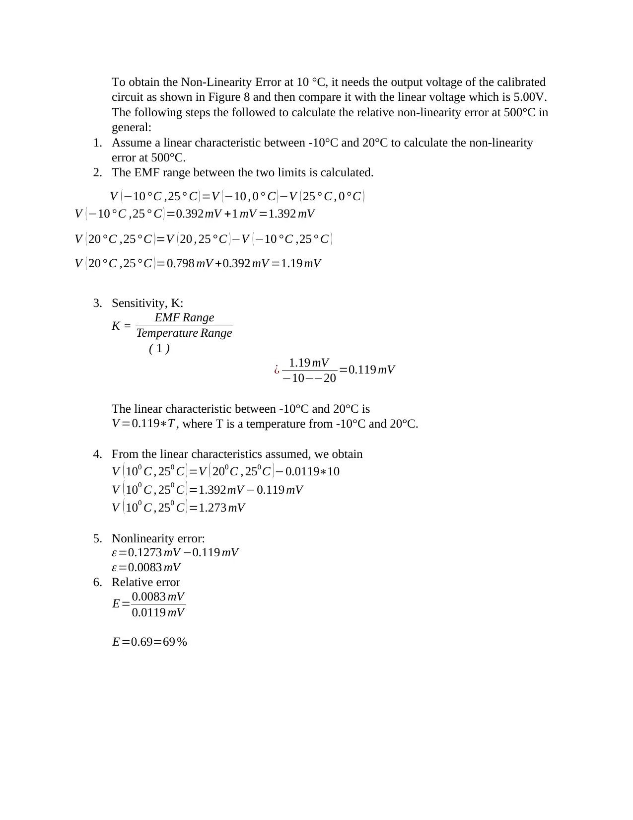
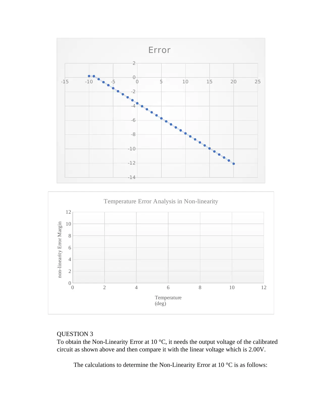
This assignment focuses on the analysis of a thermistor-based temperature sensor circuit, including the use of an op-amp 741. The solution utilizes Multisim software to simulate and analyze the circuit's behavior across a temperature range of -100°C to 200°C. It details the circuit specifications, including thermistor characteristics and desired output voltage range. The assignment addresses several key questions, such as calculating resistance values, determining non-linearity errors, and improving the circuit's performance. The analysis involves calculating voltage outputs, non-linearity errors, and sensitivity. The assignment also explores the impact of gain and offset adjustments on non-linearity. The document provides tables and figures to illustrate the circuit's performance and the effects of various parameters on the output voltage. The conclusion summarizes the key findings and emphasizes the importance of thermistor selection and circuit design in achieving accurate temperature measurements.

UNIVERSITY AFFILIATION
FACULTY OR DEPARTMENT
COURSE NAME
COURSE ID
TITLE:
SENSORS AND MEASUREMENT
STUDENT NAME
STUDENT REGISTRATION ID
PROFESSOR (TUTOR)
DATE OF SUBMISSION

Coursework Task Sheet

LIST OF FIGURES
Figure 1 Non-Inverting Operational Amplifier opamp-741..........................................................3
Figure 2 The Circuit Schematic of the OpAmp-741 and controller Circuit.......................................4
Figure 3 Circuit OpAmp 741 and controller circuit...................................................................5
Figure 4 For the highest temperature value measured.................................................................7
Figure 5 The circuit connection with a temperature sensor and thermistor.....................................12
Figure 6 The non-linearity maximum output of the system improvement by 25%............................14
Figure 7 This is the maximum output that can be obtained at non-linearity of 75%..........................15
Figure 8 The output voltage of 200C after Non-linearity improvement by 50%...............................16
LIST OF TABLES
Table 1 Non-Linearity Errors of the original Calibration as used in the Question 1 above..................14

INTRODUCTION
A thermistor is a type of resistor used to measure temperature changes, relying on the change in
its resistance with changing temperature. The thermistor is a combination of the words thermal
and change. Thermistors are made of semiconductor materials such as the metallic compounds
including oxides such as manganese, copper, cobalt, and nickel, as well as single-crystal
semiconductors silicon and germanium. Thermistors can be classified on the basis of the constant
k. when K is positive, the resistance increases with increasing temperature, and the device is
called a positive temperature coefficient, PTC and when it is negative, the resistance decreases
with increasing temperature and the corresponding device is the negative temperature coefficient.
CIRCUIT SPECIFICATIONS
Thermistor 44007
Temperature Range -100C to +200C
Output -1.0 V to +2.0V
Output Tolerance ± 5 mV
Type of OpAmp 741
DC Powers ± 12V
± 100 mV
Type of amplifier in your circuit Inverting amplifier
Tolerance of resistance due to aging and
environment variations
± 1% of normal value
Accuracy of the Thermistor ± 1% of normal value
Reference Temperature: 250C
Figure 1 Non-Inverting Operational Amplifier opamp-741
QUESTION 1
Using the Multisim Software, the circuit was obtained as shown in the diagram below,

Figure 2 The Circuit Schematic of the OpAmp-741 and controller Circuit
In most process applications the temperature sensor is inserted into a thermowell or protection
tube. To obtain the output voltage range as minimum and maximum value of the components
from the charts of the thermistor model 440007.
The range of resistance,
R¿=27.67 k −6.247 k =21.423 ohms
The temperature range of -100C to 200C.
The circuit tuning is done by adjusting the sensor resistance value to get the output as intended.
The key space switches from one mode to the next with a maximum temperature of 20 degrees
recording an output voltage of 2V and a minimum temperature of -10 degrees recording an
output of 1V.

Figure 3 Circuit OpAmp 741 and controller circuit
The circuit snippet demonstrates the connection of the non-inverting operational amplifier
connected to the controller circuit. The minimum voltage output is obtained as 1 Volts as
required of the thermistor model 440007.
To obtain the different resistance and temperature equivalents on the circuit with a voltage output
range of 1v- 2v.
The value of the Rt, sensor resistor, is obtained as,
Noninverting Amplifier Gain , Av= Range of Output Voltage
Range of Input Voltage
Range of Output Voltage=2−1=1 V
The input resistance range,
R¿=27.67 k −6.247 k =21.423 k
Measuring the resistance, one can use the Steinhart-Hart equation to calculate the temperature
from the resistance,
1
T = A+Bln ( R ) +C [ ln ( R ) ]3
The output resistance,
Rout =10 Kohm

Noninverting Amplifier Gain , Av= 10 k
21.423 k
Noninverting Amplifier Gain , Av=0.46679≅ 0.47
V out =−V ref ( R2
R1 )+V ¿ (1+ R2
R1 )
1=−V ref ( R2
100 )+ 0.00119 (1+ R2
100 )
10=−V ref ( R2
100 ) +0.0 1273 ( 1+ R2
100 )
Therefore;
V ref =( 10−0.01273− (0.01273 x 10−2 R2 ))
−10−2 R2
Substituting V ref in equation (2)
1=−10−0.01273−(0.01273 x 10−2 R2 )
−10−2 R2
( R2
100 ) +0.00119 ( 1+ R2
100 )
1=10−0.01273− ( 0.01273 x 10−2 R2 ) + 0.00119+(0.00119 x 10−2 R2 )
1=9.98727− ( 0.01392 x 10−2 R2 )
R2= ( 9.98727−1 )
0.01392 x 10−2 = 8.98727
0.0001392 =6456.372 Ω
R3=is a reverse control resistor
From the previous calculations, R2= 6456.372 Ω which equals 64.563% of the 100k ohms.
From these calculations one can obtain the following chart,

Figure 4 For the highest temperature value measured
V ( 25 °C ,0 ° C ) =1.000 mV ; V ( −10 ° C ,0 ° C ) =−0.392 mV ; V ( 20 °C ,0 ° C ) =0.798 mV
V ( T 1 ,T 2 )=V ( T 1 , 0° C )−V (T 2 , 0 °C ) (1)
Using equation 1, we have the following:
V (−10 ° C ,25 ° C ) =V (−10 , 0 ° C )−V ( 25 ° C , 0 °C )
V (−10 ° C ,25 ° C ) =0.392mV +1 mV =1.392 mV
V ( 20 °C ,25 ° C )=V ( 20 , 25 °C )−V (−10 °C ,25 ° C )
V ( 20 ° C ,25 ° C ) =0.798 mV +0.392 mV =1.19 mV
The output results are obtained as,

T
(°C)
Equivalent
EMF Reference
Input Voltage
(mV)
Linear
Voltage Output
Voltage (V)
Differenc
e
Non-
Linearity
(mV) 25° EMF
(mV) (V) ΔV Error
(%)
(V)
-10 0.392 1.754 0.798 1 1.001 0.203 0.11571
-9 0.431 1.754 0.8436 1.05 1.031 0.1874 0.106818
-8 0.47 1.754 1.2996 1.1 1.065 -0.2346 -0.133722
-7 0.508 1.754 1.7556 1.15 1.099 -0.6566 -0.374262
-6 0.547 1.754 2.2116 1.2 1.133 -1.0786 -0.614802
-5 0.586 1.754 2.6676 1.25 1.167 -1.5006 -0.855342
-4 0.624 1.754 3.1236 1.3 1.201 -1.9226 -1.095882
-3 0.663 1.754 3.5796 1.35 1.235 -2.3446 -1.336422
-2 0.701 1.754 4.0356 1.4 1.269 -2.7666 -1.576962
-1 0.739 1.754 4.4916 1.45 1.303 -3.1886 -1.817502
0 0.778 1.754 4.9476 1.5 1.337 -3.6106 -2.058042
1 0.817 1.754 5.4036 1.55 1.371 -4.0326 -2.298582
2 0.856 1.754 5.8596 1.6 1.405 -4.4546 -2.539122
3 0.895 1.754 6.3156 1.65 1.439 -4.8766 -2.779662
4 0.934 1.754 6.7716 1.7 1.473 -5.2986 -3.020202
5 0.973 1.754 7.2276 1.75 1.507 -5.7206 -3.260742
6 1.012 1.754 7.6836 1.8 1.541 -6.1426 -3.501282
7 1.051 1.754 8.1396 1.85 1.575 -6.5646 -3.741822

8 1.09 1.754 8.5956 1.9 1.609 -6.9866 -3.982362
9 1.129 1.754 9.0516 1.95 1.643 -7.4086 -4.222902
10 1.168 1.754 9.5076 2 1.677 -7.8306 -4.463442
11 1.207 1.754 9.9636 2.05 1.711 -8.2526 -4.703982
12 1.246 1.754 10.4196 2.1 1.745 -8.6746 -4.944522
13 1.285 1.754 10.8756 2.15 1.779 -9.0966 -5.185062
14 1.324 1.754 11.3316 2.2 1.813 -9.5186 -5.425602
15 1.363 1.754 11.7876 2.25 1.847 -9.9406 -5.666142
16 1.402 1.754 12.2436 2.3 1.881 -10.3626 -5.906682
17 1.441 1.754 12.6996 2.35 1.915 -10.7846 -6.147222
18 1.48 1.754 13.1556 2.4 1.949 -11.2066 -6.387762
19 1.519 1.754 13.6116 2.45 1.983 -11.6286 -6.628302
20 1.558 1.754 14.0676 2.5 1.9864 -12.0812 -6.886284
QUESTION 2
-15 -10 -5 0 5 10 15 20 25
-300
-250
-200
-150
-100
-50
0
50
100
150
200
f(x) = 8.47 x
R² = 0.37
Output Voltage(Vo) against Temperature (deg)
Temperature (deg)
Output Voltage
Non-linearity maximum error range,

To obtain the Non-Linearity Error at 10 °C, it needs the output voltage of the calibrated
circuit as shown in Figure 8 and then compare it with the linear voltage which is 5.00V.
The following steps the followed to calculate the relative non-linearity error at 500°C in
general:
1. Assume a linear characteristic between -10°C and 20°C to calculate the non-linearity
error at 500°C.
2. The EMF range between the two limits is calculated.
V ( −10 °C ,25 ° C ) =V ( −10 , 0 ° C ) −V ( 25 ° C , 0 °C )
V (−10 ° C ,25 ° C ) =0.392mV +1 mV =1.392 mV
V ( 20 °C ,25 ° C )=V ( 20 , 25 °C )−V (−10 °C ,25 ° C )
V ( 20 ° C ,25 ° C ) =0.798 mV +0.392 mV =1.19 mV
3. Sensitivity, K:
K = EMF Range
Temperature Range
( 1 )
¿ 1.19 mV
−10−−20 =0.119 mV
The linear characteristic between -10°C and 20°C is
V =0.119∗T , where T is a temperature from -10°C and 20°C.
4. From the linear characteristics assumed, we obtain
V ( 100 C , 250 C )=V ( 200 C , 250 C )−0.0119∗10
V ( 100 C , 250 C )=1.392mV −0.119 mV
V ( 100 C , 250 C ) =1.273 mV
5. Nonlinearity error:
ε =0.1273 mV −0.119 mV
ε =0.0083 mV
6. Relative error
E=0.0083 mV
0.0119 mV
E=0.69=69 %

-15 -10 -5 0 5 10 15 20 25
-14
-12
-10
-8
-6
-4
-2
0
2
Error
0 2 4 6 8 10 12
0
2
4
6
8
10
12
Temperature Error Analysis in Non-linearity
Temperature
(deg)
non-linearity Error Margin
QUESTION 3
To obtain the Non-Linearity Error at 10 °C, it needs the output voltage of the calibrated
circuit as shown above and then compare it with the linear voltage which is 2.00V.
The calculations to determine the Non-Linearity Error at 10 °C is as follows: