Short Selling's Impact on Earnings Management: An Experiment

The provided document is a research paper titled "Short Selling and Earnings Management: A Controlled Experiment" published in the Journal of Finance. The study, conducted during the SEC's pilot program (2005-2007) where some stocks were exempt from short-sale price tests, investigates the impact of short selling on corporate financial reporting. The research reveals that pilot firms exhibited decreased discretionary accruals and a lower likelihood of marginally beating earnings targets. Moreover, these firms were more likely to be caught for pre-existing fraud and showed improved stock price efficiency in incorporating earnings information. The findings suggest that short selling, or the prospect of it, acts as a constraint on earnings management, aids in fraud detection, and enhances price efficiency. The paper contributes to the literature by demonstrating the influence of short selling on financial reporting, identifying it as a determinant of earnings management, highlighting its role in improving price efficiency, and adding to the policy debate surrounding the benefits and costs of short selling.

THE JOURNAL OF FINANCE • VOL. LXXI, NO. 3 • JUNE 2016
Short Selling and Earnings Management:
A Controlled Experiment
VIVIAN W. FANG, ALLEN H. HUANG, and JONATHAN M. KARPOFF ∗
ABSTRACT
During 2005 to 2007,the SEC ordered a pilot program in which one-third of the
Russell 3000 index were arbitrarily chosen as pilot stocks and exempted from short-
sale price tests. Pilot firms’ discretionary accruals and likelihood of marginally beating
earnings targets decrease during this period, and revert to pre-experiment levels when
the program ends. After the program starts, pilot firms are more likely to be caught
for fraud initiated before the program,and their stock returns better incorporate
earnings information. These results indicate that short selling, or its prospect, curbs
earnings management, helps detect fraud, and improves price efficiency.
PREVIOUS RESEARCH SHOWS that short sellers can identify earnings manipulation
and fraud before they are publicly revealed.1 But this is for earnings manip-
ulation that has already taken place. Might short selling also constrain firms’
incentives to manipulate or misrepresent earnings in the first place? That is,
does the prospect of short selling help improve the quality of firms’financial
reporting?
In this paper we exploit a randomized experiment that allows us to address
this question.In July 2004, the Securities and Exchange Commission (SEC)
adopted a new regulation governing short-selling activities in the U.S. equity
markets–Regulation SHO.Regulation SHO contained a Rule 202T pilot pro-
gram in which stocks in the Russell 3000 index were ranked by trading volume
∗Fang is with the University of Minnesota.Huang is with the Hong Kong University of Sci-
ence and Technology.Karpoff is with the University of Washington.We are grateful for helpful
comments from two anonymous referees, an anonymous Associate Editor, Kenneth Singleton (the
Editor), Vikas Agarwal, Mark Chen, John Core, Hemang Desai, Jarrad Harford, Adam Kolasin-
ski, Craig Lewis, Paul Ma, Scott Richardson,Ed Swanson, Jake Thornock, Wendy Wilson,and
seminar participants at the Cheung Kong Graduate School of Business,Peking University, the
SEC/Maryland Conference on the Regulation of Financial Markets, the CEAR/GSU Finance Sym-
posium on Corporate ControlMechanisms and Risk, the FARS Midyear Meeting, the HKUST
Accounting Symposium,the CFEA Conference,and the UC Berkeley Multi-disciplinary Confer-
ence on Fraud and Misconduct.We are grateful to Russell Investments for providing the list of
2004 Russell 3000 index firms, and to Jerry Martin for providing the KKLM data on financial mis-
representation. Huang gratefully acknowledges financial support from a grant from the Research
Grants Council of the HKSAR, China (Project No. HKUST691213).
1 See Dechow, Sloan, and Sweeney (1996), Christophe, Ferri, and Angel (2004), Efendi, Kinney,
and Swanson (2005),Desai, Krishnamurthy, and Venkataraman (2006),and Karpoff and Lou
(2010).
DOI: 10.1111/jofi.12369
1251

1252 The Journal of FinanceR
within each exchange and every third one was designated as a pilot stock.
From May 2, 2005 to August 6, 2007, pilot stocks were exempted from short-
sale price tests, including the tick test for exchange-listed stocks and the bid
test for NASDAQ National Market (NASDAQ-NM) stocks.2
The pilot program creates an idealsetting to examine the effect ofshort
selling on corporate financial reporting decisions, for three reasons. First, the
exemption from short-sale price tests decreased the cost ofshort selling in
the pilot stocks relative to the nonpilot stocks (SEC (2007), Diether, Lee, and
Werner (2009)). The pilot program thus eliminates the need to directly estimate
short-selling costs, a notoriously difficult task (Lamont (2012)). Rather, we use
the fact that the prospect of short selling increased for pilot firms relative to
nonpilot firms during the program. Second, the pilot program represents a truly
exogenous shock to the cost of selling short in the affected firms. We identify no
evidence that the firms themselves lobbied for the pilot program, or that any
individual firm could know it would be in the pilot group until the program was
announced. Third, the pilot program had specific beginning and ending dates,
facilitating difference-in-differences (hereafter, DiD) analysis of the impact of
short-selling costs on firms’financial reporting. In particular, the anticipated
ending date allows us to investigate whether the effects of the pilot program
reversed when it ended – an important check on the internal validity of the
DiD tests (e.g., Roberts and Whited (2013)).
We begin by verifying that pilot firms represent a random draw from the Rus-
sell 3000 population. In the fiscal year before the pilot program, pilot and non-
pilot firms are similar in size, growth, investment, profitability, leverage, and
dividend payout. Although the two groups of firms also exhibit similar levels of
discretionary accruals before the program, pilot firms significantly reduce their
signed discretionary accruals once the program starts.3 After the program ends,
pilot firms’discretionary accruals revert to pre-program levels.The nonpilot
firms, meanwhile, show no significant change in discretionary accruals around
the pilot program. Our point estimates indicate that performance-matched dis-
cretionary accruals, as a percentage of assets, are one percentage point lower
for pilot firms than for nonpilot firms during the pilot program compared to
the pre-pilot period.This corresponds to 7.4% ofthe standard deviation of
discretionary accruals in our sample.
We also examine the pilot program’s effect on two alternative measures of
earnings management. First, we find that the likelihood of beating the analyst
2 The pilot program was originally scheduled to commence on January 3,2005,and end on
December 31,2005 (Securities Exchange Act Release No.50104,July 28, 2004).However,the
SEC postponed the commencement date to May 2, 2005 (Securities and Exchange Act Release No.
50747, November 29, 2004) and extended the end date to August 6, 2007 (Securities and Exchange
Act Release No. 53684, April 20, 2006). Before the pilot program ran its entire course, the SEC
eliminated short-sale price tests for all exchange-listed stocks on July 6, 2007 (Securities Exchange
Act of 1934 Release No. 34-55970, July 3, 2007).
3 Following the literature (e.g., Kothari, Leone, and Wasley (2005)), we measure discretionary ac-
cruals as the difference between actual accruals and a benchmark estimated within each industry-
year. Details are provided in Section II.C.

Short Selling and Earnings Management 1253
consensus forecast by up to one cent is 1.8 percentage points lower for the pilot
firms than for the nonpilot firms during the pilot program compared to the pre-
pilot period. This represents 11.1% of the unconditional likelihood of meeting
or just beating the analyst consensus forecast in our sample.Similarly, the
likelihood of meeting or just beating the firm’s quarterly earnings per share
(EPS) in the same quarter of the prior year is 0.8 percentage points lower
for the pilot firms during the pilot program compared to the pre-pilot period,
representing 14.2% of the unconditional likelihood.Second,we find that the
likelihood of being classified as a misstating firm,based on the F-score of
Dechow et al. (2011), is significantly lower for the pilot firms during the pilot
period compared to the pre-pilot period. Combined with our results regarding
discretionary accruals, these results indicate that pilot firms decrease earnings
management during the pilot program.
We consider several alternative interpretations for the patterns we observe
in discretionary accruals. One possibility is that pilot firms’ discretionary accru-
als reflect changes in their growth, investment, or equity issuance, as Grullon,
Michenaud, and Weston (2015) document a significant reduction in financially
constrained pilot firms’investment and equity issuance during the pilot pro-
gram. We consider several ways to control for firm growth and investment, both
in the construction of our discretionary accruals measures and in the multivari-
ate tests. None of these controls have a material effect on our main findings.
We also find that the pilot firms’ investment levels do not follow a pattern that
would explain the changes in their discretionary accruals during and after the
pilot program. Regarding the possible impact of equity issuance, we find that
pilot firms’discretionary accruals pattern is similar between firms that do not
seek to issue equity and the overall sample.These results indicate that the
effect of the pilot program on discretionary accruals is unlikely to be explained
by changes in pilot firms’growth, investment, or equity issuance around the
program.
Another possible explanation is that managers of the pilot firms decreased
earnings management because of a general increase in the attention investors
paid to these firms.Using three measures of market attention,however,we
do not find that pilot firms were subject to greater attention during the pilot
program.In multivariate DiD tests, the market attention measures are not
significantly related to discretionary accruals,nor do they affect our main
findings regarding discretionary accruals.
The most plausible interpretation of our results is that the pilot program
reduced the cost of short selling sufficiently among the pilot firms to increase
potential short sellers’ monitoring activities, and that the increased monitoring
induced a decrease in these firms’earnings management.4 We conduct three
additional tests to further probe this interpretation. First, we find that, among
the pilot firms during the pilot program, short selling is positively related to
signed discretionary accruals. Second, we find that short interest increases in
4 Throughout this paper, we use “potentialshort sellers” or “short sellers” to refer to both
investors who may take new short positions and investors with existing short positions.

1254 The Journal of FinanceR
months in which firms are later revealed to have engaged in financial misrepre-
sentation during our sample period. And third, we find that, among firms that
previously initiated financial fraud,pilot firms are more likely to get caught
than control firms after the pilot period started.We also find that the un-
conditional likelihood of pilot firms being caught for financial fraud converges
monotonically toward that of nonpilot firms as we sequentially include cases of
fraud initiated after the pilot program begins. This result is consistent with the
argument that pilot firms’conditional likelihood of being caught for any fraud
they commit is higher during the program, and with our main finding that pilot
firms endogenously adjust by decreasing earnings manipulation after the pilot
program begins.
Finally, we examine the implications of the pilot program for price efficiency
through its effect on firms’ reporting practices. We show that the coefficients of
pilot firms’ current returns on future earnings increase during the pilot period.
Among firms announcing particularly negative earnings surprises,the well-
documented post-earnings announcement drift (PEAD)disappears for pilot
firms during the period, while it remains significant for nonpilot firms. These
results indicate that the reduction in pilot firms’ earnings management during
the pilot program corresponds to an increase in the efficiency of their stock
prices as their stock returns better incorporate earnings information.
The above findings make four contributions to the literature. First, they show
that an increase in the prospect of short selling has a significant effect on firms’
financial reporting. This result demonstrates one avenue through which trad-
ing in secondary financial markets affects firms’decisions.5 Second, our find-
ings identify a new determinant of earnings management, namely, short-sale
constraints, adding to the factors identified in prior research (for a review, see
Dechow, Ge, and Schrand (2010)). Third, our results indicate that the prospect
of short selling improves price efficiency not only by facilitating the flow of
private information into prices (e.g., Miller (1977), Harrison and Kreps (1978),
Chang, Cheng, and Yu (2007), Boehmer and Wu (2013)), but also by decreasing
managers’tendency to manage earnings. And fourth, our findings contribute
to the policy debate on the benefits and costs of short selling. Previous research
demonstrates that short sellers are good at identifying the overpriced shares
of firms that have manipulated earnings, and short sellers’ trading accelerates
the discovery of financial misconduct.6 Our results indicate that the prospect
of short selling conveys additional external benefits to investors by improving
financial reporting quality and stock price efficiency in general,even among
firms not charged with financial reporting violations.
5 See Bond, Edmans, and Goldstein (2012) for a survey of research on the real effects of financial
markets. For example, Karpoff and Rice (1989) and Fang, Noe, and Tice (2009) examine the effect
of stock liquidity on firm performance, Fang, Tian, and Tice (2014) examine the effect of liquidity
on innovation,and Grullon, Michenaud, and Weston (2015) examine the effect of short-selling
constraints on investment and equity issuance.
6 See the references in footnote 1. To be sure, other studies have noted the potential dark side of
short selling, as manipulative short selling could reduce price efficiency (e.g., Gerard and Nanda
(1993), Henry and Koski (2010)).

Short Selling and Earnings Management 1255
This paper is organized as follows. Section I describes short-sale price tests in
the U.S. equity markets, how they can affect firms’tendency to manage earn-
ings, and related research.Section II describes the data.Section III reports
tests of the effect of Regulation SHO’s pilot program on firms’earnings man-
agement. Section IV examines whether short sellers actually increased their
scrutiny of the pilot stocks during the pilot program by comparing the prob-
ability of fraud detection between pilot and nonpilot firms. Section V reports
on tests that examine whether the pilot program coincided with an increase
in the efficiency of pilot firms’stock prices with respect to earnings.Finally,
Section VI concludes.
I. Short-Sale Price Tests, Their Effect on Earnings Management, and
Related Research
A. Short-Sale Price Tests in U.S. Equity Markets
Short-sale price tests were initially introduced in the U.S. equity markets in
the 1930s, ostensibly to avoid bear raids by short sellers in declining markets.
The NYSE adopted an uptick rule in 1935,which was replaced in 1938 by a
stricter SEC rule, Rule 10a-1,also known as the “tick test.” The latter rule
mandates that a short sale can only occur at a price above the most recently
traded price (plus tick) or at the most recently traded price if that price exceeds
the last different price (zero-plus tick).7 In 1994, the National Association of
Securities Dealers (NASD) adopted its own price test (the “bid test”) under Rule
3350. Rule 3350 requires that a short sale occur at a price one penny above the
bid price if the bid is a downtick from the previous bid.8
To facilitate research on the effects ofshort-sale price tests on financial
markets, the SEC initiated a pilot program under Rule 202T of Regulation
SHO in July 2004. Under the pilot program, every third stock in the Russell
3000 index ranked by trading volume within each exchange was selected as a
pilot stock. From May 2, 2005, to August 6, 2007, pilot stocks were exempted
from short-sale price tests. The program effectively ended one month early on
July 6, 2007, when the SEC eliminated short-sale price tests for all exchange-
listed stocks including the nonpilot stocks.
The decision to eliminate all short-sale price tests prompted a huge back-
lash from managers and politicians.In 2008, NYSE Euronext commissioned
Opinion Research Corporation (2008)to conduct a study to seek corporate
7 Narrow exceptions apply, as specified in SEC’s Rule 10a-1, section (e).
8 Rule 3350 applies to NASDAQ National Market (NASDAQ-NM or NNM) securities. Securities
traded in the OTC markets, including NASDAQ Small Cap, OTCBB, and OTC Pink Sheets, are
exempted. When NASDAQ became a national listed exchange in August 2006, NASD Rule 3350
was replaced by NASDAQ Rule 3350 for NASDAQ Global Market securities (formerly NASDAQ-
NM securities) traded on NASDAQ, and NASD Rule 5100 for NASDAQ-NM securities traded over
the counter. The NASDAQ switched from fractional pricing to decimal pricing over the March 12,
2001 to April 9, 2001 period. Prior to decimalization, Rule 3350 required a short sale to occur at a
price 1/8th of a dollar (if before June 2, 1997) or 1/16th of a dollar (if after June 2, 1997) above the
bid.

1256 The Journal of FinanceR
issuers’views on short selling. Fully 85% of the surveyed corporate managers
favored reinstituting the short-sale price tests “as soon as practical,” indicating
that managers are aware of and sensitive to the impact of eliminating price
tests on the potential amount of short selling in their firms. The former state
banking superintendent of New York argued that the SEC’s repeal of the price
tests added to market volatility, especially in down markets.9 The Wall Street
Journal argued that SEC (2007) was too biased to evaluate the short-sale price
tests fairly.10 Wachtell, Lipton, Rosen & Katz, a well-known law firm, argued
that the uptick rule should be reinstated immediately,and three members
of Congress introduced a bill (H.R.6517) requiring the SEC to reinstate the
uptick rule. Presidential candidate Sen. John McCain blamed the SEC for the
recent financial turmoil by “turning our markets into a casino,” in part because
of the increased prospect of short sales, and called for the SEC’s chairman to
be dismissed. In response to this pressure, the SEC partially reversed course
and restored a modified uptick rule on February 24, 2010. Under the new rule,
price tests are triggered when a security’s price declines by 10% or more from
the previous day’s closing price. This policy reversal drew sharp criticism itself,
this time from hedge funds and short sellers.11
B. The Impact of the Pilot Program on Earnings Management
The strong public reactions to changes in the uptick rule indicate that the
rule is important to investors, managers, and politicians. Consistent with prac-
titioners’perception, most prior research indicates that short-sale price tests
impose meaningfulconstraints on short selling,an assumption we examine
further in the next section.12 In this section, we draw from prior studies to
construct our main hypothesis on how changes in the cost of short selling due
to the removal of short-sale price tests, and the corresponding changes in the
prospect of short selling,affect a manager’s tendency to engage in earnings
management.
Previous research indicates that executives have incentives to distort their
firms’ reported financial performance to bolster their compensation,gains
through stock sales, job security, operational flexibility, or control.13 These find-
ings imply that managers can earn a personal benefit from managing earnings
9 Gretchen Morgenson, “Why the roller coaster seems wilder,” The New York Times, August 26,
2007, page 31.
10 See “There’s a better way to prevent bear raids,” The Wall Street Journal, November 18, 2008,
page A19.
11 See “Hedge funds slam short-sale rule,” available at http://dealbook.nytimes.com/2010/02/
25/hedge-funds-slam-short-sale-rule/? r=0.
12 See, for example, McCormick and Reilly (1996), Angel (1997), Alexander and Peterson (1999,
2008),SEC (2007),and Diether,Lee, and Werner (2009).For a contradictory finding,see Ferri,
Christophe, and Angel (2004).
13 For evidence regarding compensation motives, see Bergstresser and Philippon (2006), Burns
and Kedia (2006), and Efendi, Srivastava, and Swanson (2007); for stock sale motives, see Beneish
and Vargus (2002); and for job security and control-related motives, see DeFond and Park (1997),
Ahmed, Lobo, and Zhou (2006), DeFond and Jiambalvo (1994), and Sweeney (1994).

Short Selling and Earnings Management 1257
to inflate the stock price.Prior research also demonstrates that short sell-
ing facilitates the flow of unfavorable information into stock prices, increases
price efficiency,and dampens the price inflation that motivates managers to
manipulate earnings in the first place (e.g., Miller (1977), Harrison and Kreps
(1978), Chang, Cheng, and Yu (2007), Karpoff and Lou (2010), Boehmer and Wu
(2013)). These findings imply that managers’ benefits of manipulating earnings
decrease with the prospect of short selling because these benefits are at least
partially offset by short sellers’activities.
Although earnings management conveys benefits to managers,managers
cannot manipulate earnings with impunity. Previous research shows that ag-
gressive earnings management is associated with an increased likelihood of
forced CEO turnover (Karpoff, Lee, and Martin (2008), Hazarika, Karpoff, and
Nahata (2012)), and that short sellers monitor managers’reporting behavior
and uncover aggressive earnings management (Efendi, Kinney, and Swanson
(2005),Desai, Krishnamurthy, and Venkataraman (2006),Karpoff and Lou
(2010)). These results indicate that, for a given level of earnings management,
managers’potential costs increase with a reduction in the cost of short selling
and an increase in short sellers’scrutiny.
Regulation SHO’s pilot program, which eliminated short-sale price tests for
the pilot stocks,represents an exogenously imposed reduction in the cost of
short selling and hence an increase in the prospect of short selling in these
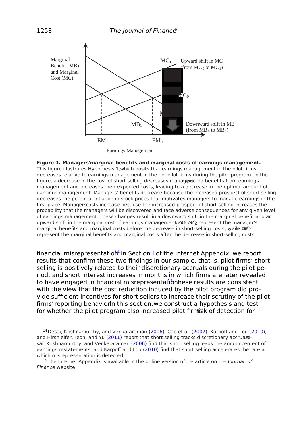
stocks. The effect was to decrease pilot firm managers’expected benefits and
increase their expected costs of earnings management. These effects on a man-
ager’s earnings management decisions are illustrated in Figure 1. Let MB0 and
MC 0 represent the manager’s marginal benefit and marginal cost of managing
earnings before initiation of the pilot program. In drawing these curves with
their normal slopes,we assume that the benefits from artificialstock price
inflation increase at a decreasing rate in the level of earnings management,
while the costs from the prospect of being discovered increase at an increas-
ing rate. The pre-program optimum amount of earnings management is EM0.
Once the program starts, the marginal benefit and marginal cost of earnings
management shift to MB1 and MC1, and the manager endogenously adjusts by
choosing a new,lower level of earnings management,EM 1. This adjustment
among pilot firms leads to our first hypothesis:
HYPOTHESIS 1: Earnings management in the pilot firms decreases relative to
earnings management in the nonpilot firms during the pilot program.
C. The Impact of the Pilot Program on Fraud Discovery
In developing Hypothesis 1,we assume that the pilot program had a sub-
stantial enough effect on short sellers’ activities to induce a measurable change
in the pilot firms’financial reporting decisions. Previous research finds that,
in general, short selling tracks firms’ discretionary accruals and helps uncover

1258 The Journal of FinanceR
MC1
MC0
MB1
MB0
Marginal
Benefit (MB)
and Marginal
Cost (MC)
Earnings Management
EM0EM1
M
MB0
Upward shift in MC
(from MC 0 to MC1)
Downward shift in MB
(from MB 0 to MB1)
Figure 1. Managers’marginal benefits and marginal costs of earnings management.
This figure illustrates Hypothesis 1,which posits that earnings management in the pilot firms
decreases relative to earnings management in the nonpilot firms during the pilot program. In the
figure, a decrease in the cost of short selling decreases managers’expected benefits from earnings
management and increases their expected costs, leading to a decrease in the optimal amount of
earnings management. Managers’ benefits decrease because the increased prospect of short selling
decreases the potential inflation in stock prices that motivates managers to manage earnings in the
first place. Managers’costs increase because the increased prospect of short selling increases the
probability that the managers will be discovered and face adverse consequences for any given level
of earnings management. These changes result in a downward shift in the marginal benefit and an
upward shift in the marginal cost of earnings management. MB0 and MC0 represent the manager’s
marginal benefits and marginal costs before the decrease in short-selling costs, while MB1 and MC1
represent the marginal benefits and marginal costs after the decrease in short-selling costs.
financial misrepresentation.14 In Section I of the Internet Appendix, we report
results that confirm these two findings in our sample, that is, pilot firms’ short
selling is positively related to their discretionary accruals during the pilot pe-
riod, and short interest increases in months in which firms are later revealed
to have engaged in financial misrepresentation.15 These results are consistent
with the view that the cost reduction induced by the pilot program did pro-
vide sufficient incentives for short sellers to increase their scrutiny of the pilot
firms’ reporting behavior.In this section,we construct a hypothesis and test
for whether the pilot program also increased pilot firms’risk of detection for
14 Desai, Krishnamurthy, and Venkataraman (2006), Cao et al. (2007), Karpoff and Lou (2010),
and Hirshleifer, Teoh, and Yu (2011) report that short selling tracks discretionary accruals.De-
sai, Krishnamurthy, and Venkataraman (2006) find that short selling leads the announcement of
earnings restatements, and Karpoff and Lou (2010) find that short selling accelerates the rate at
which misrepresentation is detected.
15 The Internet Appendix is available in the online version of the article on the Journal of
Finance website.

Short Selling and Earnings Management 1259
earnings manipulation that rises to the level of financial misrepresentation or
fraud.16
We begin by noting that there is generally a time lag between when a firm
begins misrepresenting its earnings and when the misrepresentation is de-
tected.Karpoff and Lou (2010)report that this lag varies across firms and
has a median of 26 months in their sample. We therefore characterize a firm’s
conditional probability of being caught as
Pr (Caught(t + n) |Fraud (t)) = δ n
s=0msSSP (t + s) . (1)
In equation (1), Pr(Caught(t + n)|Fraud(t)) is the firm’s probability of being
caught at time t + n conditional on misrepresenting at time t, where n ࣙ 0. On
the right-hand side, SSP(t + s) is short selling potential at time t + s; we expect
this potential to be higher for pilot firms when t + s falls within the pilot period.
We use ms to denote the individual weight each period’s short-selling potential
contributes to the conditional probability of detection. This weight depends on
the wide range of non short-selling factors that affect a firm’s probability of
being caught. We hypothesize that an increase in short-selling potential helps
uncover aggressive reporting, that is, δ > 0. This leads to our second hypothesis:
HYPOTHESIS 2: Conditional on misreporting,pilot firms are more likely than
nonpilot firms to get caught after the pilot program begins.
A challenge in testing Hypothesis 2 is that we do not directly observe the
conditional probability of detection,but rather the unconditional probability
that a firm both commits fraud and is detected, which can be expressed as
Pr Caught(t + n) , Fraud (t) = Pr (Fraud (t))× Pr Caught(t + n) |Fraud (t) . (2)
To test Hypothesis 2, we exploit the time lag between the commission and
detection of fraud. Since the pilot firms are randomly selected, it is reasonable
to assume that, before the pilot program was announced in July 2004, the actual
rate of fraud commission was equal between the pilot and nonpilot firms, that
is, Pr(Fraud(t))pilot = Pr(Fraud(t))nonpilot for t < July 2004.17 This allows us to
use the unconditional probability of detection for fraud initiated before the pilot
program was announced in July 2004 but detected after the program began in
May 2005 to infer the conditional probability of getting caught. Hypothesis 2
then implies that
Pr (Caught(post-May 2005) , Fraud (pre-July 2004))pilot >
Pr (Caught(post-May 2005) , Fraud (pre-July 2004))nonpilot.
16 Karpoff et al. (2016) point out that many instances of financial misrepresentation do not in-
clude charges of fraud. We nonetheless use the term “fraud” to refer to any illegal misrepresentation
that attracts SEC enforcement action.
17 We restrict t to the period before the announcement of the pilot program (in July 2004) to
ensure that the expected rate of fraud commission is equal across the two groups of firms. Whereas
short sellers arguably begin to change their behavior after the pilot program is implemented in
May 2005, managers of pilot firms could change their reporting behavior in response to the prospect
of short selling as early as when they learn the identity of the pilot stocks in July 2004.

1260 The Journal of FinanceR
Once the pilot program was announced, Hypothesis 1 implies that managers
of the pilot firms endogenously began to adjust to the higher conditional prob-
ability of detection by decreasing earnings management, that is,
Pr (Fraud (t))pilot < Pr (Fraud (t))nonpilot for t > July 2004.
The pilot program therefore has two offsetting effects on the unconditional
probability of detection for fraud committed after July 2004: pilot firms commit
fewer frauds, but conditional on committing fraud, they are more likely to be
caught.This implies that the difference between pilot and nonpilot firms in
the unconditional likelihood of fraud detection should decrease as we consider
fraud initiated after July 2004. Section IV reports results that support these
implications of Hypothesis 2.
D. Related Research
Our investigation is related to the small but growing literature that exploits
changes in short-sale regulations to examine the economic implications of short
selling. Autore, Billingsley, and Kovacs (2011), Frino, Lecce, and Lepone (2011),
and Boehmer, Jones, and Zhang (2013) examine the impact of a widespread ban
on short selling in U.S. equity markets in 2008, and Beber and Pagano (2013)
examine the impacts ofshort-selling bans around the world.These studies
conclude that short-selling bans decrease various measures of market quality.
Using Regulation SHO’s Rule 202T pilot program, Alexander and Peterson
(2008)find that order execution and market quality improved for the pilot
stocks during the pilot program.Diether, Lee, and Werner (2009) and SEC
(2007) show that pilot stocks listed on both NYSE and NASDAQ experienced a
significant increase in short-sale trades and in the ratio of short sales to share
volume during the term of the pilot program. The former also shows that NYSE-
listed pilot stocks experienced a higher level of order-splitting, suggesting that
short sellers apply more active trading strategies.Other papers relate the
pilot program to firm outcomes.Grullon, Michenaud,and Weston (2015),for
example,examine the effect of the pilot program on pilot firms’stock prices,
equity issuance, and investment. Kecsk´es, Mansi, and Zhang (2013) study bond
yields, De Angelis, Grullon, and Michenaud (2015) equity incentives, He and
Tian (2014) corporate innovation,and Li and Zhang (2015) firms’voluntary
disclosure practices.
In our main analyses, we use the experiment created by the pilot program
to examine the effect ofshort-selling costs on firms’earnings management
decisions.This experiment is well suited for our research question, as it
facilitates DiD comparisons of pilot vs. nonpilot firms’earnings management
before, during, and after the pilot program. The DiD tests allow us to control
for time trends that may be common to both the pilot and nonpilot firms,
and mitigate concerns about reverse causality or omitted variables (because
the SEC assigned pilot stocks arbitrarily).This experimental design is thus
superior to a blanket ban of short selling that applies to the entire cross-section

Short Selling and Earnings Management 1261
of firms because the latter can be muddled by possible confounding events. For
example, changes in accruals following the blanket ban on short selling during
the recent financial crisis could be associated with economy-wide changes in
investment opportunities rather than changes in short-selling regulations.
A contemporaneous paper by Massa, Zhang, and Zhang (MZZ, 2015) also in-
vestigates the effects of short selling on firms’ earnings management. Whereas
we use the exogenous variation in firms’ short-selling costs created by the pilot
program to identify our tests, MZZ focus on 33 international markets and use
the amount of shares available for lending to measure short-selling potential.
Like us, MZZ also infer that short selling plays a disciplinary role in deterring
firms’opportunistic reporting behavior.
II. Data
A. Sample
On July 28, 2004, the SEC issued its first pilot order (Securities Exchange
Act Release No.50104) and published a list of 986 stocks that would trade
without being subject to any price tests during the term of the pilot program
(available at http://www.sec.gov/rules/other/34-50104.htm). To create this list,
the SEC started with 2004 Russell 3000 index members and excluded stocks
that were not previously subject to price tests (i.e., not listed on NYSE, Amex,
or NASDAQ-NM) and stocks that went public or had spin-offs after April 30,
2004.The remaining stocks were then sorted by their average daily dollar
volume computed over the June 2003 to May 2004 period within each of the
three listing markets. Every third stock (beginning with the second one) within
each listing market was designated as a pilot stock.
Based on the description in the SEC’s pilot orders and its report on the pilot
program (SEC (2007)),we identify an initial sample of 986 pilot stocks and
1,966 nonpilot stocks.18 An examination of the exchange distribution of these
stocks shows that both the pilot and the nonpilot groups are representative
of the Russell 3000 index,confirming the statistics reported by SEC (2007).
Specifically,of the 986 pilot stocks,49.9% (492) are listed on NYSE,47.9%
(472) on NASDAQ-NM, and 2.2% (22) on Amex. The exchange distribution of
nonpilot stocks is very similar, with 50% (982) listed on NYSE, 48% (944) on
NASDAQ-NM, and 2% (40) on Amex.
In our tests, we delete firms in the financial services (SIC 6000–6999)
and utilities (SIC 4900–4949) industries because disclosure requirements,
18 We use Thomson Reuters’s Securities Data Company (SDC) Platinum database and the Com-
pustat database to identify firms that went public or had spinoffs after April 30,2004,and the
CRSP monthly files to identify stocks that are not exchange-listed,and exclude all such stocks
from the nonpilot sample.The SEC did not publish the final list of nonpilot stocks in its 2007
analysis, but any discrepancies between the SEC’s sample and our sample of nonpilot stocks are
likely to be immaterial. Further, firms that are not exchange-listed or that had significant changes
in ownership structure around the pilot program are likely to be excluded from our tests because
our main tests require that the sample firms have financial data each year from 2001 to 2003
(inclusive) and 2005 to 2010 (inclusive).

1262 The Journal of FinanceR
accounting rules,and processes by which accruals are generated are signif-
icantly different for these regulated industries.A further complication with
financial stocks is the 2008 short-sale ban imposed on this sector.We obtain
data from the Compustat Industrial Annual Files to construct earnings man-
agement proxies and controlvariables.In most tests, we require that firms
have data to calculate firm characteristics over the entire sample period, that
is, 2001 to 2003 (inclusive) and 2005 to 2010 (inclusive). The resulting balanced
panel sample consists of 388 pilot firms and 709 nonpilot firms. If we relax this
requirement, our unbalanced panel sample contains 741 to 782 pilot firms and
1,504 to 1,610 nonpilot firms in the year immediately before the announcement
of the pilot program (i.e., 2003), depending on data availability to calculate a
given firm characteristic.We emphasize the results from the balanced panel
sample,but also report results for the unbalanced sample.Throughout,the
results are similar using either sample.
B. Key Test Variables
We create an indicator variable PILOT to denote firms with pilot stocks
(“pilot firms”). Specifically, PILOT equals one if a firm’s stock is designated as
a pilot stock under Regulation SHO’s pilot program and zero otherwise. Pilot
firms constitute the treatment sample and nonpilot firms serve as the control
sample. The sample period in our main analysis consists of nine calendar
years, 2001 to 2003 (inclusive) and 2005 to 2010 (inclusive). We construct three
variables to indicate three subperiods:PRE equals one if a firm-year’s fiscal
end falls between January 1, 2001 and December 31, 2003 and zero otherwise;
DURING equals one if a firm-year’s fiscal end falls between January 1, 2005
and December 31,2007 and zero otherwise;and POST equals one if a firm-
year’s fiscal end falls between January 1, 2008 and December 31, 2010 and zero
otherwise. We set the subperiods to three calendar years each so it is easier to
align and compare firm financials across periods in the DiD tests,especially
since our outcome variable of interest, earnings quality, exhibits seasonality.
Our during-pilot period, 2005 to 2007, is slightly longer than the course of
the pilot program,which was scheduled to run from May 2,2005 to August
6, 2007 but effectively ran from May 2,2005 to July 6, 2007.This definition
of DURING reflects our assumption that firms’annual reporting outcome is
affected even if the increased prospect of short selling does not extend for the
full year. Table IA.III of the Internet Appendix reports tests that yield similar
results if we instead define the three subperiods as May 2001 to June 2003, May
2005 to June 2007, and May 2008 to June 2010, thus restricting the DURING
period more closely to the actualstart and end dates of the program.Also,
in our primary DiD tests, we omit 2004 because the identity of the pilot and
nonpilot stocks was made public in July 2004, and it is not clear whether 2004
should be classified as part of the pre- or during-pilot period. In Table IA.IV of
the Internet Appendix, we report tests that indicate our main findings are not
substantially affected if we include the entire year of 2004 in the PRE period

Short Selling and Earnings Management 1263
or Q1 to Q3 of 2004 in the PRE period and Q4 in the DURING period (as most
of Q4’s financial statements would be released in calendar year 2005).
C. Measures of Earnings Management
Our primary proxy for earnings management is the performance-matched
discretionary accruals measure of Kothari, Leone, and Wasley (2005). To con-
struct this measure, we first estimate the following cross-sectional model within
each fiscal year and Fama-French 48 industry:
TAi,t
ASSET i,t−1
= β0 + β1
1
ASSET i,t−1
+ β2
REV i,t
ASSET i,t−1
+ β3
PPE i,t
ASSET i,t−1
+ εi,t , (3)
where i indexes firms and t indexes fiscal years. Total accruals TAt are defined
as earnings before extraordinary items and discontinued operations minus
operating cash flows for fiscal year t;ASSET t−1 is total assets at the end of
year t−1; REV t is the change in sales revenue from year t−1 to t; and PPEt
is the gross value of property, plant, and equipment at the end of year t. We
require at least 10 observations to perform each cross-sectional estimation.
Next, we use the following model and the estimated coefficients from
equation (3) to compute the fitted normal accruals NAi,t:
NA i,t = β0 + β1
1
ASSET i,t−1
+ β2
REV i,t − AR i,t
ASSET i,t−1
+ β3
P PE i,t
ASSET i,t−1
. (4)
Following Dechow, Sloan, and Sweeney (1995), the change in accounts receiv-
able is subtracted from the change in sales revenue as credit sales might also
provide a potential opportunity for accounting distortion. After obtaining the
fitted normal accruals NAi,t from equation (4), we calculate firm-year-specific
discretionary accruals as DAi,t = (TAi,t / ASSET i,t−1) − NAi,t.
Finally, we adjust the estimated discretionary accruals for performance. We
match each sample firm with the firm from the same fiscal year-industry that
has the closest return on assets as the given firm. The performance-matched
discretionary accruals, denoted as Discretionary accruals, are then calculated
as the firm-specific discretionary accruals minus the discretionary accruals of
the matched firm. Note that Discretionary accruals is signed and constructed
to be positively related to income-increasing earnings management.19
D. Firm Characteristics
Similar to Grullon, Michenaud,and Weston (2015),we compare pilot and
nonpilot firms’characteristics in the fiscalyear immediately before the an-
nouncement of the pilot program, 2003.Table I, Panel A, reports descriptive
statistics for the balanced panel sample, in which we require that firms have
19 We create three additional performance-matched discretionary accrual measures by removing
the intercept term from equations (3) and (4) and/or replacing
REV i,t
ASSET i,t−1 with (REV i,t −AR i,t )
ASSET i,t−1 in

1264 The Journal of FinanceR
Table I
Firm Characteristics of the Treatment and Control Groups in Fiscal
Year 2003
Panel A and Panel B report summary statistics of the firm characteristics for the balanced and the
unbalanced panel sample of the treatment and control groups, respectively. All characteristics are
measured in 2003, the year immediately before Regulation SHO’s pilot program was announced.
The balanced sample comes from the 2004 Russell 3000 index and contains firms that have data
available to calculate firm characteristics and discretionary accruals over the entire sample period
(i.e., annual data from 2001 to 2003 and 2005 to 2010). The unbalanced sample is similar to the
balanced sample but only requires data to be available to calculate a firm characteristic of interest
in a given year. A firm is classified into the treatment group if its stock is designated as a pilot
stock during the program and into the control group otherwise. Variable definitions are provided
in the Appendix. All variables are winsorized at the 1% and 99% levels. ASSET is in millions of
dollars. ASSETGR, CAPEX, R&D, ROA, CFO, LEV, CASH, and DIVIDENDS are in percentage
points.***, **, and* indicate significance at the 1%, 5%, and 10% levels using two-tailed tests.
Panel A: Treatment and Control Groups in the Balanced Panel Sample
Treatment Group (PILOT = 1) Control Group (PILOT = 0)
N Mean Median SD N Mean Median SD
ASSET 388 3,748.61 817.69 8,512.30 709 3,746.25 817.42 8,647.29
MB 388 2.75 1.95 3.79 709 2.60 1.98 3.13
ASSETGR 388 13.42 7.88 31.28 709 13.22 7.66 30.18
CAPEX 388 5.55 3.76 5.54 709 5.50 3.65 5.88
R&D 388 4.19 0.00 8.40 709 4.04 0.32 7.83
ROA 388 14.37 14.51 12.70 709 14.15 14.29 14.30
CFO 388 11.36 11.33 10.68 709 10.56 10.46 13.26
LEV 388 29.36 26.46 27.50 709 29.80 27.56 28.25
CASH 388 21.07 12.22 25.76 709 21.81 10.66 27.87
DIVIDENDS 388 0.83 0.00 1.49 709 0.73 0.00 1.33
Tests for differences between PILOT = 1 and PILOT = 0
t-statistic Wilcoxon z-statistic
ASSET 0.00 0.51
MB 0.68 0.03
ASSETGR 0.10 −0.30
CAPEX 0.14 0.91
R&D 0.27 −0.94
ROA 0.25 0.22
CFO 1.10 1.10
LEV −0.25 −0.24
CASH −0.44 −0.32
DIVIDENDS 1.14 1.07
(Continued)
data available to calculate financial characteristics and accrual measures in
all years of the sample period. The mean book value of assets in both groups
equation (3). The results using these alternative measures are reported in Table IA.V of the Internet
Appendix and are consistent with those reported in the paper.

Short Selling and Earnings Management 1265
Table I—Continued
Panel B: Treatment and Control Groups in the Unbalanced Panel Sample
Treatment Group (PILOT = 1) Control Group (PILOT = 0)
N Mean Median SD N Mean Median SD
ASSET 782 2,918.37 726.92 7,471.08 1,610 2,941.31 669.22 7,883.20
MB 759 2.66 1.89 3.84 1,534 2.55 1.85 4.15
ASSETGR 781 17.81 8.82 40.64 1,605 17.61 8.45 43.10
CAPEX 741 5.59 3.61 6.21 1,504 5.28 3.31 5.98
R&D 781 5.78 0.00 11.96 1,605 6.10 0.22 12.22
ROA 778 10.67 12.79 18.92 1,604 9.68 11.87 20.88
CFO 742 8.19 9.88 17.20 1,505 7.20 9.24 19.20
LEV 781 30.82 28.06 29.18 1,602 31.54 27.27 31.21
CASH 781 26.45 13.03 35.86 1,605 27.17 12.17 37.37
DIVIDENDS 778 0.73 0.00 1.55 1,600 0.77 0.00 1.65
Tests for differences between PILOT = 1 and PILOT = 0
t-statistic Wilcoxon z-statistic
ASSET −0.07 1.26
MB 0.60 1.05
ASSETGR 0.11 0.38
CAPEX 1.13 1.74*
R&D −0.61 −1.06
ROA 1.15 1.23
CFO 1.23 1.39
LEV −0.55 0.11
CASH −0.48 −0.66
DIVIDENDS −0.69 −1.13
is $3.7 billion. The two groups also exhibit similar mean and median values of
the market-to-book ratio, one-year growth in assets, capital expenditures to as-
sets, R&D expenditures to assets, annual return on assets, cash flow to assets,
leverage,and the levels of cash and dividends (both as a percentage of total
assets). In none of these comparisons is the difference statistically significant,
which supports our argument that Regulation SHO’s pilot program is a well-
controlled experiment that is suitable for examining the effects of short-sale
constraints.
Panel B of Table I reports similar comparisons for the larger unbalanced
panel sample. Firms in this sample are slightly smaller than those in the
balanced panel sample, with assets averaging $2.9 billion versus $3.7 billion.
As in Panel A, the pilot and nonpilot firms in the unbalanced panel sample
are similar to each other along the financial characteristics we examine. The
sole exception is that the median capital expenditure of pilot firms is slightly
higher than that of nonpilot firms.

1266 The Journal of FinanceR
III. The Effect of Regulation SHO’s Pilot Program on Earnings
Management
A. Discretionary Accruals
Table II reports the results of univariate DiD tests examining Hypothesis 1
using our primary measure of earnings management based on discretionary
accruals. Panel A reports results for the balanced panel sample defined in Sec-
tion II.A. The mean Discretionary accruals during the three-year period before
the pilot program (2001 to 2003) is −0.004 for both pilot and nonpilot firms.
The t-statistic for the difference in means (i.e.,the cross-sectional estimator
−0.001) is −0.03, and the Wilcoxon z-statistic for the difference in medians is
0.77, both insignificant. During the three-year period of the pilot program (2005
to 2007), the mean Discretionary accruals decreases to −0.014 for pilot firms
while it remains at −0.004 for nonpilot firms. The mean difference is −0.011
(t-statistic = −2.09) and the median difference is −0.008 (Wilcoxon z-statistic =
−2.23), both significant at the 5% level. For the three-year period after the pi-
lot program (2008 to 2010), Discretionary accruals increases for the pilot firms
to a mean of zero while it changes slightly for the nonpilot firms to −0.003.
The mean difference is 0.004 (t-statistic = 0.69) and the median difference is
0.001 (Wilcoxon z-statistic = 0.66),both insignificant.The bottom-left cell of
Table II, Panel A, reports the time-series estimators, which track the change in
Discretionary accruals within each group of firms across the three periods. The
second column shows that the average Discretionary accruals for pilot firms
drops by −0.011 (significant at the 5% level) from the pre- to during-pilot pe-
riod, but increases by 0.013 (significant at the 1% level) after the program ends.
Consistent with this reverting pattern, the time-series estimator comparing pi-
lot firms’ average Discretionary accruals from the pre- to post-pilot period is
0.003 and insignificant.In contrast, the estimators in the fourth column are
never significant, suggesting that nonpilot firms’ Discretionary accruals do not
change much over time.
The bottom-right cellof Table II, Panel A, reports results on the DiD es-
timators.The mean DiD estimator for Discretionary accruals from before to
during the pilot program is −0.011 with a t-statistic of −1.67. This difference is
statistically significant at the 10% level. However, the results from other tests
reported below, including multivariate DiD tests and the results from the un-
balanced panel, are significant at lower levels. The DiD estimator that tracks
Discretionary accruals from during to after the pilot program is 0.013 with a
t-statistic of 2.06. In addition, the DiD estimator that compares Discretionary
accruals pre-program to post-program is statistically insignificant with a t-
statistic of 0.32. The last two DiD estimators demonstrate that the effect of the
pilot program on discretionary accruals reverses when the program ends–an
important check on the internal validity of the DiD test.
We plot these univariate results in Figure 2 to better illustrate the pattern
in discretionary accruals.As the figure shows,nonpilot firms’discretionary
accruals do not change much over the sample period. The pilot firms’discre-
tionary accruals, similar to those of the nonpilot firms before the pilot program,

Short Selling and Earnings Management 1267
Table II
Discretionary Accruals before, during, and after the Pilot Program
The top half of Panel A reports summary statistics on the level of annual discretionary accruals for the balanced panel sample of the treatment and
control groups for the three-year periods before, during, and after Regulation SHO’s pilot program, and differences in the mean or median. The bottom
half of Panel A reports univariate results of difference-in-differences (DiD) tests. The sample comes from the 2004 Russell 3000 index and contains
firms that have data available to calculate firm characteristics and discretionary accruals over the entire sample period (i.e., 2001 to 2003 (inclusive)
and 2005 to 2010 (inclusive)). A firm is classified into the treatment group if its stock is designated as a pilot stock during the program and into the
control group otherwise. Panel B reports summary statistics on the level of discretionary accruals for the unbalanced panel sample of the treatment
and control groups. This sample also comes from the 2004 Russell 3000 index and contains firms that have data available to calculate discretionary
accruals in a given year. Variable definitions are provided in the Appendix.***, **, and * indicate significance at the 1%, 5%, and 10% levels using
two-tailed tests.
Panel A: Balanced Panel Sample
Treatment Group (PILOT = 1) Control Group (PILOT = 0) Cross-Sectional Estimator
N Mean Median N Mean Median Difference in Mean Difference in Median
Discretionary accruals
PRE (2001-2003) 1,164 −0.004 −0.001 2,127 −0.004 −0.003 −0.001 0.002
DURING (2005-2007) 1,164 −0.014 −0.012 2,127 −0.004 −0.004 −0.011** −0.008**
POST (2008-2010) 1,164 0.000 0.000 2,127 −0.003 −0.001 0.004 0.001
Univariate DiD test N Time-Series Estimator N Time-Series Estimator DiD Estimator t-statistic
Discretionary accruals
DURING-PRE 388 −0.011** 709 0.000 −0.011 −1.67*
POST-DURING 388 0.013*** 709 0.001 0.013 2.06**
POST-PRE 388 0.003 709 0.001 0.002 0.32
Treatment Group (PILOT = 1) Control Group (PILOT = 0) Cross-Sectional Estimator
N Mean Median N Mean Median Difference in Mean Difference in Median
Panel B: Unbalanced Panel Sample
Discretionary accruals
PRE (2001-2003) 2,067 −0.002 0.000 4,151 0.000 −0.002 −0.002 0.002
DURING (2005-2007) 1,865 −0.012 −0.009 3,740 −0.003 −0.003 −0.009** −0.006**
POST (2008-2010) 1,605 0.001 0.001 3,087 −0.005 −0.003 0.006 0.004

1268 The Journal of FinanceR
-0.016
-0.014
-0.012
-0.010
-0.008
-0.006
-0.004
-0.002
0.000
0.002
Pre-pilot During-pilot Post-pilot
Discreonary Accruals of Pilot Firms
Discreonary Accruals of Nonpilot Firms
Figure 2. Discretionary accruals for pilot vs.nonpilot firms.This figure displays the re-
sults reported in Panel A of Table II. It depicts the mean Discretionary accruals for the balanced
panel sample of the treatment group and control group for the periods before, during, and after
Regulation SHO’s pilot program, that is, 2001 to 2003, 2005 to 2007, and 2008 to 2010. The sample
comes from the 2004 Russell 3000 index and contains firms that have data available to calculate
financial characteristics and discretionary accruals over the entire sample period (i.e., 2001 to 2003
(inclusive) and 2005 to 2010 (inclusive)).
decrease significantly during the program and then revert to levels that are
similar to those of the nonpilot firms after the program.
Panel B of Table II reports on the changes in Discretionary accruals using
data from the unbalanced panel sample, in which we do not require that firms
have financial data available for all years of the sample period. The results are
similar to those from the balanced panel sample even though we are only able
to calculate the cross-sectional estimators given the unbalanced sample.
Next, we extend the DiD test using multivariate regressions.To do so,we
retain firm-year observations for both pilot and nonpilot firms for the nine-
year window (2001 to 2003 (inclusive) and 2005 to 2010 (inclusive)) around
Regulation SHO’s pilot program and estimate the following model:
Discretionary accrualsi,t = β0 + β1PILOT i × DURING t + β2PILOT i
× POST t + β3PILOT i + β4DURING t + β5POST t + εi,t . (5)
The variables are as defined in Sections II.B and II.C. The benchmark pe-
riod consists of the three years before the pilot program (2001 to 2003).As
previously discussed,2004 is omitted from these tests because the identity
of the pilot stocks was announced midway through 2004.The regression re-
sults estimating equation (5) are reported in column (1) of Table III. The co-
efficients of interest are the two DiD estimators,β1 and β2. The coefficient
on PILOT×DURING, β1, is negative and significant at the 5% level. The

Short Selling and Earnings Management 1269
Table III
The Effect of Pilot Program on Discretionary Accruals
This table reports OLS regression results on differences in pilot and nonpilot firms’discretionary
accruals for the periods before, during, and after Regulation SHO’s pilot program, using a balanced
panel sample. The sample comes from the 2004 Russell 3000 index and contains firms that have
data available to calculate firm characteristics and discretionary accruals over the entire sample
period (i.e.,2001 to 2003 (inclusive) and 2005 to 2010 (inclusive)).A firm is classified into the
treatment group if its stock is designated as a pilot stock during the program and into the control
group otherwise. We estimate the following model using annual data: Discretionary accrualsi,t =
β0 + β1PILOT i ×DURING t + β2PILOT i ×POST t + β3PILOT i + β4DURING t + β5POST t + εi,t
in column (1). We augment the model by including SIZE, MB, ROA, and LEV in column (2) and
by further including year fixed effects for 2002 to 2003 and 2005 to 2010 in column (3). We omit
PILOT and POST in column (3) to avoid multicollinearity. Variable definitions are provided in the
Appendix. Standard errors clustered by year and firm are displayed in parentheses. For brevity,
the coefficient estimates on year fixed effects in column (3) are not reported.***, **, and * indicate
significance at the 1%, 5%, and 10% levels using two-tailed tests.
Discretionary accrualst
(1) (2) (3)
PILOT×DURING t −0.010** −0.010** −0.010**
(0.004) (0.004) (0.004)
PILOT×POST t 0.004 0.003 0.003
(0.004) (0.004) (0.005)
PILOT −0.000 0.000 0.000
(0.003) (0.003) (0.003)
DURING t −0.001 −0.001
(0.002) (0.002)
POST t 0.000 −0.001
(0.005) (0.005)
SIZE t 0.002* 0.002*
(0.001) (0.001)
MB t −0.001 −0.001
(0.001) (0.001)
ROAt −0.041** −0.041***
(0.016) (0.016)
LEV t −0.014 −0.013
(0.009) (0.008)
INTERCEPT −0.004** −0.006 −0.006
(0.002) (0.007) (0.008)
Year fixed effects Included
No. of obs. 9,873 9,873 9,873
Adjusted R2 0.10% 0.40% 0.40%
magnitude of β1 is consistent with the univariate DiD results reported in Ta-
ble II and indicates that Discretionary accruals (i.e., discretionary accruals as
a percentage of total assets) is one percentage point lower for the treatment
group than for the control group during the three-year period of the pilot pro-
gram compared to the three-year pre-pilot period. This corresponds to 7.4% of
the standard deviation of Discretionary accruals in the pooled sample, 0.135.

1270 The Journal of FinanceR
The coefficient on PILOT×POST, β2, is insignificant. This result once again
demonstrates a reverting pattern because the difference between the pilot and
non-pilot firms’discretionary accruals after the pilot program is not statisti-
cally different from that before the program. Also, the coefficient on PILOT, β3,
is insignificant, indicating that pilot and nonpilot firms exhibit similar levels of
discretionary accruals before the pilot program. Consistent with prior research,
the regression R2 is low, indicating that most of the cross-sectional differences
in discretionary accruals are due to unmodeled factors.
In column (2), we augment equation (5) by including four controls previously
shown to affect a firm’s level of discretionary accruals (e.g.,Kothari, Leone,
and Wasley (2005), Zang (2012)): the natural logarithm of total assets (SIZE),
market-to-book (MB), return on assets (ROA), and leverage (LEV). In column
(3), we further include year fixed effects from 2002 to 2003 and from 2005 to
2010, but omit DURING and POST as well as the fixed effect for 2001 (the base
year) to avoid multicollinearity. The results are similar when we include these
additional controls.
B. Alternative Measures
In this section, we examine whether our results based on discretionary ac-
cruals are robust to using two alternative measures of earnings management.
First, we examine whether the pilot program differentially affected firms’ likeli-
hood of meeting or marginally beating the analyst consensus forecast. Graham,
Harvey, and Rajgopal (2005) report that a large majority of CFOs consider it
important to beat the analyst consensus forecast and are willing to engage in
earnings manipulation to do so.For this reason, many papers (e.g.,Bhojraj
et al. (2009)) infer earnings management from the tendency of firms to meet or
beat the analyst consensus by up to one cent.
We follow prior research and run the following probit model on a panel of
quarterly earnings announcements that take place during the same nine-year
window (2001 to 2003 (inclusive) and 2005 to 2010 (inclusive)):
BEAT ALY i,q = β0 + β1PILOT i × DURING q + β2PILOT i × POSTq
+ β3PILOT i + β4DURING q + β5 POST q + εi,q . (6)
Subscript q indexes fiscal quarters.The dependent variable BEAT ALY is
coded one for quarters in which the firm’s reported EPS meets or beats the
most recent analyst consensus EPS forecast before the earnings announce-
ment by up to one cent. Both reported EPS and analyst forecasts are retrieved
from I/B/E/S. To calculate analyst consensus,we take each analyst’s latest
forecast issued within 90 days of the fiscal quarter-end and before the earn-
ings announcement, and require a firm-quarter to have at least three analysts.
We define PILOT as before but the two time indicators are now based on the
earnings announcement date, that is, DURINGq (POST q) equals one if quarter

Short Selling and Earnings Management 1271
q’s earnings announcement takes place during (post) the pilot period, and zero
otherwise.
The regression results estimating equation (6) are reported in column
(1) of Table IV. Consistent with our earlier results using discretionary ac-
cruals, the coefficienton our main variable of interest–the DiD estimator
(PILOT×DURING) – is negative and significant at the 5% level. The marginal
effect of β1, calculated using the methodology suggested in Aiand Norton
(2003), indicates that the likelihood of marginally beating the analyst consen-
sus is 1.8 percentage points lower for the treatment group than for the control
group during the three-year period of the pilot program compared to the three-
year pre-pilot period. This corresponds to 11.1% of the unconditional likelihood
of BEAT ALY in the sample, 16.2%.20 The coefficient on the second DiD es-
timator (PILOT×POST), β 2, continues to be insignificant, indicating that the
difference between pilot and nonpilot firms’ likelihood of marginally beating the
analyst consensus in the post-pilot period is not statistically different from that
pre-pilot. The coefficient on PILOT, β3, also remains insignificant, consistent
with pilot firms and nonpilot firms having a similar likelihood of marginally
beating the analyst consensus pre-pilot.
In column (2), we include a list of controls previously shown to affect the like-
lihood of beating the analyst consensus. We largely follow Edmans, Fang, and
Lewellen (2015) to construct these controls, which include the log of market cap-
italization (MV), market-to-book (MB), return on assets (ROA), the log of ana-
lyst coverage (ALY N), the log of the average forecast horizon (ALY HORIZON),
and analyst forecast dispersion (ALY DISP).We also include two proxies for
real earnings management: the change in R&D expenditures from quarter q−4
to quarter q, R&D q, and the change in capital expenditures, CAPEXq, both
scaled by total assets at the beginning of quarter q. Among these controls, the
market-to-book ratio is positively related to the likelihood of marginally beat-
ing the analyst consensus while forecast horizon, forecast dispersion, and an
increase in R&D spending are negatively related to this likelihood. The inclu-
sion of these controls, however, does not significantly alter the magnitude or
significance of the coefficients on the pilot-related variables.
The time dummy variables DURING and POST both exhibit significantly
negative coefficients in columns (1)and (2). This result is consistent with
the view that Regulation FD in 2000 reduced firms’ability to guide analyst
forecasts toward reported earnings. In Table IA.VI of the Internet Appendix,
we repeat the analysis including quarterly fixed effects to control for secular
changes in firms’tendency to meet or marginally beat the analyst consensus
forecast. The results, particularly for the pilot-related variables, are similar to
those reported in Table IV.
20 Ai and Norton (2003) argue that the magnitude of the interaction effect in nonlinear regres-
sions may not equal its marginal effect and propose a way to correct for the interaction term’s
magnitude and standard error. Le (1998) and Kolasinski and Siegel (2010), however, argue that
the coefficient on the interaction term is relevant even in a nonlinear regression, especially when
used to measure proportional rather than absolute marginal effects. In our setting, the interaction
effect calculated using the conventional linear method is only slightly larger (2% vs. 1.8%).

1272 The Journal of FinanceR
Table IV
The Effect of Pilot Program on Firm’s Likelihood of Beating Earnings
Targets
This table reports probit regression results on differences in pilot and nonpilot firms’likelihood of
meeting or marginally beating the quarterly analyst consensus forecast (or the reported earnings
for the same quarter of the prior year) for the periods before, during, and after Regulation SHO’s
pilot program. The sample comes from the 2004 Russell 3000 index and contains firms that have
data available for analyst forecast related variables (or reported EPS in the same quarter of the
prior year), and controls during the sample period (i.e., 2001 to 2003 (inclusive) and 2005 to 2010
(inclusive)). A firm is classified into the treatment group if its stock is designated as a pilot stock
during the program and into the control group otherwise. We estimate the following model using
quarterly data: BEAT ALY (BEAT EPS) i,q = β0 + β1PILOT i ×DURING q + β2PILOT i ×POST q +
β3PILOT i + β4DURING q + β5POST q + εi,q in column (1) (column (3)). We augment the model by
including MV, MB, ROA, ALY N, ALY HORIZON, ALY DISP, R&D, and CAPEX in column (2)
and MV, MB, ROA, R&D, and CAPEX in column (4). Variable definitions are provided in the
Appendix. Standard errors clustered by quarter-end and firm are displayed in parentheses.***, **,
and * indicate significance at the 1%, 5%, and 10% levels using two-tailed tests.
BEAT ALY q BEAT EPS q
(1) (2) (3) (4)
PILOT×DURING q −0.081** −0.079** −0.073* −0.074*
(0.040) (0.040) (0.043) (0.044)
PILOT×POST q 0.020 0.017 0.001 −0.003
(0.043) (0.043) (0.032) (0.033)
PILOT 0.028 0.022 0.041* 0.045*
(0.028) (0.029) (0.023) (0.024)
DURING q −0.217*** −0.219*** 0.081** 0.089**
(0.048) (0.050) (0.038) (0.039)
POST q −0.461*** −0.437*** −0.072** −0.062*
(0.055) (0.056) (0.033) (0.032)
MV q 0.002 −0.065***
(0.010) (0.007)
MB q 0.018*** 0.006**
(0.003) (0.003)
ROAq −0.632 1.389***
(0.412) (0.324)
ALY N q −0.020
(0.024)
ALY HORIZON q −0.031**
(0.015)
ALY DISP q −0.202***
(0.040)
R&D q −1.865** −0.245
(0.865) (0.423)
CAPEX q −0.140 0.340
(0.988) (0.379)
INTERCEPT −0.759*** 0.680*** −1.682*** −1.233***
(0.042) (0.057) (0.024) (0.057)
No. of obs. 28,626 28,341 59,846 59,589
Pseudo R2 1.87% 2.21% 0.15% 0.64%

Short Selling and Earnings Management 1273
Graham, Harvey, and Rajgopal (2005) report that an alternative benchmark
that firms might try to beat is the firm’s EPS in the same quarter of the prior
year. We therefore repeat our tests using BEAT EPS, an indicator that equals
one if the firm’s quarterly EPS meets or beats the prior year same quarter’s
EPS by up to one cent. The results are tabulated in columns (3) and (4) of
Table IV. The results are qualitatively similar to those using BEAT ALY, al-
though the coefficients on PILOT×DURING are significant at only the 10%
level. The weaker statistical significance is consistent with Brown and Caylor’s
(2005) finding that analyst consensus, and not prior-year earnings, has become
the most important earnings target for U.S.firms in recent years.Nonethe-
less, the economic significance remains sizable, as the likelihood of marginally
beating the prior year’s same-quarter EPS is 0.8 percentage points lower for
the treatment group than for the control group during the three-year period of
the pilot program compared to the three-year pre-pilot period. This represents
a 14.2% difference based on the unconditional likelihood of BEATEPS in the
sample, which is 5.3%.
Next, we examine whether the pilot program differentially affected firms’
likelihood of being classified as a misstating firm based on the F-score.The
F-score is the predicted probability of a misstatement using fitted values from
a model developed by Dechow et al. (2011), who use the model to characterize
firms subject to SEC enforcement actions for financial misconduct that include
one or more Accounting and Auditing Enforcement Release (AAER). The model
includes balance sheet items (which are intended to capture accruals quality
and financial performance),and/or nonfinancialmeasures,off-balance-sheet
activities, and market-based measures. The advantage of this measure is that
it is correlated with an ex post indication of earnings management, namely, the
incidence of SEC enforcement action for earnings manipulation.
We calculate three versions of the F-score, F1–F3, using the three different
sets of coefficient estimates provided in Dechow et al. (2011). The first set of
coefficients is obtained from their Model (1),which includes accruals quality
and financial performance measures. The second set comes from their Model
(2), which includes all variables in Model (1) plus nonfinancial measures and
off-balance-sheet activities.The third set comes from their Model (3),which
further includes market-based measures.We then define a binary variable,
HF1, which stands for “High F-score” and equals one if the firm’s F1 is greater
than or equal to the 99th percentile of the sample.We define HF2 and HF3
similarly based on Dechow et al.’s (2011) second and third models.
The results, replacing Discretionary accruals with HF1-HF3 in equation (5),
are reported in Table V. As can be seen, the coefficients on our main DiD esti-
mator of interest, PILOT×DURING, are once again negative and significant at
the 5% level in all columns. The marginal effect in column (1) indicates that the
likelihood of being classified as a misstating firm is 0.4 percentage points lower
for the treatment group than for the control group during the three-year period
of the pilot program compared to the three-year pre-pilot period. As before, the
coefficients on PILOT are insignificant, indicating that pilot and nonpilot firms
have similar probabilities ofbeing classified as misstating firms before the

1274 The Journal of FinanceR
Table V
The Effect of Pilot Program on Firm’s Likelihood of Misstating Based
on F-Scores
This table reports probit regression results on differences in pilot and nonpilot firms’likelihood
of being classified as misstating based on F-scores of Dechow et al. (2011) for the periods before,
during, and after Regulation SHO’s pilot program. The sample comes from the 2004 Russell 3000
index and contains firms that have data available to calculate F-scores and controls over the entire
sample period (i.e., 2001 to 2003 (inclusive) and 2005 to 2010 (inclusive)). A firm is classified into
the treatment group if its stock is designated as a pilot stock during the program and into the
control group otherwise. We estimate the following model using annual data: HF1 (or HF2, HF3)i,t
= β0 + β1PILOT i ×DURING t + β2PILOT i ×POST t + β3PILOT i + β4DURING t + β5POST t + εi,t in
columns (1), (3), and (5). We augment the model by including SIZE, MB, ROA, and LEV in columns
(2), (4), and (6). Variable definitions are provided in the Appendix. Standard errors clustered by
year and firm are displayed in parentheses.***, **, and * indicate significance at the 1%, 5%, and
10% levels using two-tailed tests.
HF1t HF2 t HF3t
(1) (2) (3) (4) (5) (6)
PILOT×DURING t −0.178** −0.174** −0.189** −0.187** −0.200** −0.196**
(0.080) (0.081) (0.079) (0.080) (0.080) (0.081)
PILOT×POST t −0.177** −0.170* −0.186** −0.181** −0.169** −0.167*
(0.087) (0.088) (0.087) (0.088) (0.086) (0.087)
PILOT −0.001 −0.011 −0.006 −0.016 −0.004 −0.012
(0.035) (0.036) (0.036) (0.036) (0.038) (0.039)
DURING t −0.976*** −1.024*** −0.942*** −0.989*** −0.974*** −1.015***
(0.046) (0.047) (0.045) (0.046) (0.046) (0.046)
POST t −0.941*** −0.989*** −0.928*** −0.977*** −0.887*** −0.939***
(0.049) (0.050) (0.048) (0.050) (0.048) (0.049)
SIZE t 0.079*** 0.084*** 0.072***
(0.017) (0.017) (0.017)
MB t 0.021*** 0.020*** 0.014**
(0.006) (0.006) (0.006)
ROAt 0.093 −0.000 0.026
(0.168) (0.167) (0.170)
LEV t 0.127 0.108 0.294***
(0.084) (0.083) (0.088)
INTERCEPT −0.081*** −0.735*** −0.063*** −0.726*** −0.004 −0.628***
(0.021) (0.111) (0.022) (0.110) (0.023) (0.111)
No. of obs. 9,871 9,871 9,871 9,871 9,871 9,871
Pseudo R2 11.5% 12.5% 11.0% 12.1% 10.8% 12.0%
pilot program began. However, the results using the higher F-score variables
do differ in one respect from those using discretionary accruals or the meet
or beat measures of earnings management: the coefficients on PILOT×POST
are negative and statistically significant. This result suggests that there is a
prolonged effect of the pilot program on pilot firms’earnings quality when it is
measured by the high F-score variables. We make this inference with caution,
however, because the balance sheet items used to calculate the F-score include

Short Selling and Earnings Management 1275
accruals and other variables that can be linked to investment and growth. It is
possible that our F-score results reflect the pilot program’s effect on firm invest-
ment as well as its effect on earnings management. We address this concern
for our primary tests in Section III.C below.
C. Alternative Explanations
So far, our results indicate that the increase in the prospect of short sell-
ing due to the removalof short-sale price tests is associated with a signifi-
cant decrease in pilot firms’earnings management. Hypothesis 1 implies that
these results reflect how the prospect of short selling curbs firms’opportunis-
tic reporting behavior. In this section, we evaluate several alternatives to this
explanation.
C.1. Growth, Investment, and Equity Issuance
Grullon, Michenaud, and Weston (2015)documentthat financially con-
strained pilot firms significantly reduce their investment and equity issuance
during the pilot program. So it is possible that pilot firms’ tendency to decrease
earnings management during the pilot program reflects changes in the dif-
ference between pilot and nonpilot firms’investment and/or equity issuance
around the pilot program.This concern is particularly pertinent when dis-
cretionary accruals are used to measure earnings management, because prior
research shows that a firm’s accruals correlate with its growth (e.g., Fairfield,
Whisenant, and Yohn (2003), Zhang (2007), Wu, Zhang, and Zhang (2010)) and
its incentives to issue equity (e.g.,Friedlan (1994),Teoh, Welch, and Wong
(1998a, 1998b)).
To investigate this concern, we adopt several controls for firms’investment.
We begin by re-estimating equation (5) controlling for R&D expenditures (R&D)
and capital expenditures (CAPEX), both scaled by lagged totalassets.The
results are reported in Table VI. In column (1), we include R&D and CAPEX
separately. In column (2), we include the sum of the two, INVESTMENT. The
coefficients on the two DiD estimators, PILOT×DURING and PILOT×POST,
are barely affected by the inclusion of these controls. In columns (3) and (4),
we further include squared terms of the investment variables to account for
the possibility that the effect ofinvestment on accruals may be nonlinear.
The main results remain similar.In column (5),we modify the Jones model
by adding the market-to-book ratio to equations (3) and (4) when calculating
the performance-matched discretionary accruals.That is, total accruals are
modeled as a function of the market-to-book ratio in addition to the changes in
revenues (or revenues adjusted for accounts receivable in equation (4)) and PPE
(both scaled by total assets). The results are again similar to those reported in
Table III.
As an additional check for any investment effect on accruals,we examine
changes in the investment variables around the pilot program for the two
groups of firms. If discretionary accruals reflect only growth, investment should

1276 The Journal of FinanceR
Table VI
The Effect of Pilot Program on Discretionary Accruals Controlling
for Investment
This table reports OLS regression results on differences in pilot and nonpilot firms’discretionary
accruals for the periods before, during, and after Regulation SHO’s pilot program, using a balanced
panel sample. The sample comes from the 2004 Russell 3000 index and contains firms that have
data available to calculate firm characteristics and discretionary accruals over the entire sample
period (i.e.,2001 to 2003 (inclusive) and 2005 to 2010 (inclusive)).A firm is classified into the
treatment group if its stock is designated as a pilot stock during the program and into the control
group otherwise. We estimate the following model using annual data: Discretionary accrualsi,t = β0
+ β1PILOT i ×DURING t + β2PILOT i ×POST t + β3PILOT i + β4DURING t + β5POST t + β6SIZE i,t
+ β7MB i,t + β8ROAi,t + β9LEV i,t + εi,t. We include R&D and CAPEX in column (1), INVESTMENT
in column (2), and further include their squared terms in columns (3) and (4). In column (5), we
replace the dependent variable Discretionary accruals with Discretionary accruals MBadj. Variable
definitions are provided in the Appendix. Standard errors clustered by year and firm are displayed
in parentheses.***, **, and * indicate significance at the 1%, 5%, and 10% levels using two-tailed
tests.
Discretionary accrualst
(1) (2) (3) (4)
Discretionary
accruals
MBadj t
(5)
PILOT×DURING t −0.010** −0.010** −0.010** −0.010** −0.018***
(0.004) (0.004) (0.004) (0.004) (0.004)
PILOT×POST t 0.003 0.003 0.003 0.003 0.004
(0.005) (0.004) (0.005) (0.004) (0.006)
PILOT −0.000 −0.000 −0.000 −0.000 0.004
(0.003) (0.003) (0.003) (0.003) (0.003)
DURING t −0.001 −0.001 −0.001 −0.001 0.002
(0.002) (0.001) (0.002) (0.001) (0.002)
POST t −0.002 −0.003 −0.002 −0.003 0.001
(0.005) (0.005) (0.005) (0.005) (0.005)
SIZE t 0.001 0.001 0.001 0.001 0.001
(0.001) (0.001) (0.001) (0.001) (0.001)
MB t −0.000 −0.000 −0.000 −0.000 −0.001
(0.001) (0.001) (0.001) (0.001) (0.001)
ROAt −0.062*** −0.053*** −0.064*** −0.058*** −0.044**
(0.014) (0.015) (0.014) (0.015) (0.019)
LEV t −0.017** −0.016* −0.016* −0.015* −0.013
(0.009) (0.008) (0.009) (0.009) (0.009)
R&D t −0.001*** −0.001*
(0.000) (0.000)
CAPEX t −0.001*** −0.001**
(0.000) (0.000)
INVESTMENT t −0.001*** −0.001**
(0.000) (0.000)
R&D t 2 −0.000
(0.000)
CAPEX t 2 0.000
(0.000)
INVESTMENT t 2 −0.000
(0.000)
INTERCEPT 0.015* 0.013* 0.013* 0.010 −0.001
(0.008) (0.008) (0.008) (0.007) (0.009)
No. of obs. 9,849 9,873 9,873 9,873 9,206
Adjusted R2 1.06% 1.02% 1.10% 1.10% 0.50%

Short Selling and Earnings Management 1277
follow a pattern around the pilot program that is similar to the pattern in Dis-
cretionary accruals.In Table IA.VII of the Internet Appendix, we reestimate
equation (5) replacing Discretionary accruals with CAPEX in column (1) and
INVESTMENT in column (2). Our results in column (1) are consistent with
Grullon, Michenaud, and Weston’s (2015) finding that capital expenditures de-
creased for pilot firms relative to nonpilot firms during the pilot program. How-
ever, pilot and nonpilot firms’capital expenditures do not appear to converge
when the pilot program ends,as the coefficient on PILOT×POST is signifi-
cantly negative and of a larger magnitude than that on PILOT×DURING. We
also find no evidence that pilot firms’overall INVESTMENT decreases during
the pilot program, which is consistent with Grullon, Michenaud, and Weston’s
(2015) finding that investment decreases during the pilot program only among
the financially constrained pilot firms.
We also examine whether our findings regarding pilot firms’discretionary
accruals are concentrated among firms that seek to issue equity during our
sample period.To do so,we partition the sample according to whether firms
are likely to issue equity during the pilot period. As Kadan et al. (2009) point
out, recent equity issuance is positively correlated with the ex ante likelihood
that a firm will issue equity again. We thus classify firms that issued equity at
least once in the two prior fiscal years, as recorded in Thomson Reuters’SDC
Platinum database, as Equity Issuers, and firms that did not as Nonequity Is-
suers. As an alternative test, we also partition the sample based on whether, ex
post, the firm issues equity in the given year. This alternative approach has the
advantage of identifying Equity Issuers based on firms’ actual equity issuance.
A drawback, however, is that some potential issuers could be mistakenly clas-
sified as Nonequity Issuers if they refrain from issuing equity because of the
pilot program.
The results are reported in Table VII. The first four columns report results
when the sample is partitioned on the ex ante measure of firms’ desire to issue
equity, and the last four columns report the results using the ex post measure.
Using either partition, the coefficients on PILOT×DURING is statistically sig-
nificant only among the subsample of Nonequity Issuers.The coefficients on
PILOT×DURING for the subsample of Equity Issuers range from −0.027 to
0.006 but are not statistically significant in either panel.These results indi-
cate that the effect of the pilot program on discretionary accruals is widespread
and is not limited to firms that are likely to issue equity. Overall, the results in
this section do not support the view that the pattern in discretionary accruals
that we document is driven by changes in firms’ investment levels and/or equity
issuance.21
21 The discretionary accruals measure is industry-adjusted. As a result, it is possible that our
finding that pilot firms’discretionary accruals reverted to pre-program levels after the pilot pro-
gram could reflect changes in nonpilot firms’accruals rather than changes in pilot firms’accruals.
We examine this concern in Section III of the Internet Appendix and find that the convergence
in pilot and nonpilot firms’ discretionary accruals after the pilot program does partly reflect a
decrease in total accruals among nonpilot firms.

1278 The Journal of FinanceR
Table VII
The Effect of Pilot Program on Discretionary Accruals Partitioned on
Seasoned Equity Offering
This table reports OLS regression results on differences in pilot and nonpilot firms’discretionary
accruals for the periods before, during, and after Regulation SHO’s pilot program, separately for
the subsample of equity issuers and the subsample of nonequity issuers. The sample comes from
the 2004 Russell 3000 index and contains firms that have data available to calculate firm char-
acteristics and discretionary accruals over the entire sample period (i.e., 2001 to 2003 (inclusive)
and 2005 to 2010 (inclusive)). In columns (1)-(4), we define a firm as an Equity Issuer if the firm
issued equity at least once during the two prior fiscal years, as recorded in Thomson Reuters’s SDC
Platinum database, and as a Nonequity Issuer otherwise. In columns (5)-(8), we define a firm as an
Equity Issuer if the firm issues equity at least once during a given fiscal year, as recorded in the
Thomson Reuters Securities Data Company (SDC) Platinum database, and Nonequity Issuer oth-
erwise. A firm is classified into the treatment group if its stock is designated as a pilot stock during
the program and into the control group otherwise. We estimate the following model using annual
data: Discretionary accrualsi,t = β0 + β1PILOT i ×DURING t + β2PILOT i ×POST t + β3PILOT i +
β4DURING t + β5POST t + εi,t in columns (1), (3), (5), and (7). We augment the model by including
SIZE, MB, ROA, and LEV in columns (2), (4), (6), and (8). Variable definitions are provided in the
Appendix. Standard errors clustered by year and firm are displayed in parentheses.***, **, and *
indicate significance at the 1%, 5%, and 10% levels using two-tailed tests.
Discretionary accrualst
Partition based on past equity issuance Partition based on current equity issuance
Equity Issuers Nonequity Issuers Equity Issuers Nonequity Issuers
(1) (2) (3) (4) (5) (6) (7) (8)
PILOT×DURING t 0.004 0.006 −0.011** −0.012** −0.027 −0.020 −0.009*** −0.010***
(0.008) (0.008) (0.005) (0.005) (0.036) (0.038) (0.003) (0.003)
PILOT×POST t −0.036 −0.035 0.007 0.006 0.007 0.006 0.003 0.003
(0.028) (0.028) (0.005) (0.005) (0.052) (0.052) (0.006) (0.006)
PILOT 0.003 0.003 −0.001 −0.001 −0.016 −0.016 0.001 0.002
(0.006) (0.006) (0.004) (0.004) (0.012) (0.012) (0.002) (0.002)
DURING t −0.001 −0.002 −0.001 −0.002 −0.002 −0.009 0.000 −0.000
(0.010) (0.010) (0.002) (0.003) (0.036) (0.038) (0.001) (0.002)
POST t 0.013** 0.011 −0.001 −0.003 −0.005 −0.011 0.001 0.000
(0.006) (0.009) (0.006) (0.006) (0.014) (0.016) (0.006) (0.006)
SIZE t −0.002 0.002** −0.001 0.002**
(0.002) (0.001) (0.005) (0.001)
MB t −0.002 −0.000 −0.002 −0.001
(0.001) (0.001) (0.002) (0.001)
ROAt −0.021 −0.049*** −0.040 −0.041*
(0.040) (0.019) (0.048) (0.021)
LEV t 0.005 −0.016** 0.016 −0.016
(0.018) (0.008) (0.018) (0.010)
INTERCEPT −0.010 0.009** −0.002 −0.005 0.011** 0.023 −0.005*** −0.008
(0.009) (0.004) (0.003) (0.008) (0.004) (0.030) (0.001) (0.007)
No. of obs. 1,199 1,199 8,674 8,674 559 559 9,314 9,314
Adjusted R2 0.20% 0.60% 0.10% 0.40% 0.70% 1.40% 0.10% 0.30%

Short Selling and Earnings Management 1279
C.2. Market Attention
Another possible explanation is that the pilot program focused widespread
attention on the pilot firms and these firms decreased earnings manipulation
because of such market attention rather than any particular attention from
short sellers. To examine this hypothesis, we construct three measures of mar-
ket attention. Our first measure, Search Volume Index (SVI), comes from Da,
Engelberg, and Gao (2011) and is based on the frequency with which a stock is
searched on Google. This measure arguably reflects retail investors’ awareness
of and interest in a particular firm. Our second measure of market attention
is the number of earnings forecasts issued by sell-side financial analysts. Sell-
side financial analysts work for brokerage firms and their research is typically
funded by trading commissions paid by institutions.We conjecture that if a
pilot firm experiences an increase in attention from institutionalinvestors,
institutions’ demand for information will prompt analysts to collect more infor-
mation, leading to more frequent earnings forecasts (e.g., Jacob, Lys, and Neale
(1999)). As a third measure of market attention, we use the total trading vol-
ume in the stock. Trading volume can also increase as a result of a decrease in
the cost of short selling, but for this measure we focus on the trading volume in
the period between the identification of the pilot firms and the implementation
of the program. Presumably, an increase in trading volume before the program
was implemented is more likely to reflect an increase in investors’awareness
of the firm, whereas an increase in trading volume after the program was
implemented could reflect lower shorting costs.
If the announcement of the pilot program led to an increase in market atten-
tion, the effect should occur following the announcement of the SEC’s first pilot
order (i.e., July 28, 2004), when the pilot firms were first identified. We begin
our test by restricting focus to 2004 and calculating the DiD estimator for each
of the three attention measures from the pre-announcement period (January
1, 2004 to July 27, 2004) to the post-announcement period (July 28, 2004 to De-
cember 31, 2004). As shown in Table IA.VIII, Panel A of the Internet Appendix,
none of the market attention DiD estimators are statistically significant, indi-
cating that the announcement of the pilot program did not substantially raise
market attention for pilot firms compared to nonpilot firms.
We next repeat the univariate DiD tests over our main sample period (2001 to
2003, 2005 to 2010). Table IA.VIII, Panel B, reports the results. As can be seen,
most of the DiD estimators for changes in market attention remain statistically
insignificant. There are only two statistically significant results,regarding
changes in SVI and the number of analyst earnings forecasts between the pilot
period and the post-pilot period.These results indicate that the increase in
market attention, if any, was greater for nonpilot firms.
Finally, we reestimate equation (5) including two of our attention measures,
the number of analyst forecasts and total trading volume,as additional con-
trols. We cannot include SVI as an additional control because SVI only dates
back to 2004 whereas our main sample period starts in 2001.The results,
reported in Table IA.IX, remain similar to those in Table III.

1280 The Journal of FinanceR
Market attention is an elusive concept that is difficult to measure. Nonethe-
less, our various tests of the market attention hypothesis suggest that we can-
not attribute the patterns we document in firms’earnings management to an
increase in the overall attention paid to pilot firms during the pilot program.22
IV. The Effect of Regulation SHO’s Pilot Program on Fraud Discovery
This section reports on tests of Hypothesis 2, which holds that the conditional
likelihood of fraud detection is higher for the pilot firms. We first estimate the
following probit model at the firm level:
Pre-2004 fraud caughti = β0 + β1PILOT i + εi , (7)
where Pre-2004 fraud caught is a dummy variable that equals one if (i) a firm
is identified in the Karpoff et al. (2016) database as having initiated financial
misrepresentation before July 2004, and (ii) the misconduct is revealed after
May 2005. The variable is set to zero for firms that have never been identified
to engage in financial misconduct, or engaged in misconduct but were detected
before July 2004.23 Hypothesis 2 predicts β1 to be positive.
Equation (7) represents our cleanest test ofHypothesis 2. If we assume
that pilot and nonpilot firms are equally likely to commit fraud before the an-
nouncement of the pilot program, Hypothesis 2 implies that the unconditional
likelihood of getting caught is higher for the pilot firms. Note that we do not
require that fraud detection be limited only to the pilot period (i.e.,between
May 2005 and July 2007) because, as shown in equations (1) and (2), both the
conditional and unconditional probability of detection can remain higher for
pilot firms even after the pilot program ends.
Results estimating equation (7)are reported in column (1)of Table VIII.
Consistent with Hypothesis 2, the coefficient on PILOT is positive and signifi-
cant at the 1% level. In column (2) of Table VIII, we include the four controls
used in our previous tests, namely, the natural logarithm of total assets (SIZE),
market-to-book (MB), return on assets (ROA), and leverage (LEV). We measure
the controls in fiscal year 2003, the year immediately before the announcement
of the pilot program. Consistent with the random assignment of pilot firms, the
results are barely affected when including these controls. The marginal effect
in column (2) indicates that the unconditional probability of detection for fraud
initiated before the announcement of the pilot program (i.e., July 2004) is one
percentage point higher for the pilot firms than for the nonpilot firms, which
22 We also note that the reverting pattern we observe for discretionary accruals and for the
likelihood of marginally beating earnings targets at the end of the pilot program is not consistent
with an investor awareness or market attention hypothesis. Other studies find that, when investor
awareness increases for a particular firm, such attention persists for a prolonged period and does
not quickly revert (e.g., Chen, Noronha, and Singal (2004)).
23 Firms excluded from this analysis are those that (1) engaged in fraud before July 2004 that
was detected between July 2004 and May 2005, or (2) engaged in fraud after July 2004 that was
detected after May 2005. We identify only 32 such cases. Our results are not affected by including
these firms and coding them as having zeros for Pre-2004 fraud caught.

Short Selling and Earnings Management 1281
Table VIII
The Effect of Pilot Program on the Discovery of Financial
Misrepresentation
This table reports probit regression results on differences in pilot and nonpilot firms’likelihood
of being identified as having engaged in fraud in the Karpoff et al. (2016) database. The sample
comes from the 2004 Russell 3000 index. A firm is classified into the treatment group if its stock is
designated as a pilot stock during the program and into the control group otherwise. We estimate
the following model:Pre-2004 fraud caughti = β0 + β1PILOT i + εi in column (1).We augment
the model by including SIZE, MB, ROA, and LEV in column (2), with all controls measured at the
end of fiscal year 2003. We repeat column (2) with Pre-2005 fraud caught, Pre-2006 fraud caught,
and Pre-2007 fraud caught as the dependent variables in column (3), (4), (5), respectively. Variable
definitions are provided in the Appendix. Standard errors clustered by year and firm are displayed
in parentheses.***, **, and * indicate significance at the 1%, 5%, and 10% levels using two-tailed
tests.
Pre-2004 Pre-2005 Pre-2006 Pre-2007
Fraud Caught Fraud Caught Fraud Caught Fraud Caught
(1) (2) (3) (4) (5)
PILOT 0.202*** 0.202*** 0.193*** 0.185*** 0.142*
(0.066) (0.061) (0.062) (0.070) (0.076)
SIZE 0.086*** 0.082*** 0.076*** 0.076***
(0.027) (0.026) (0.024) (0.016)
MB −0.007 0.008 0.006 0.006
(0.017) (0.014) (0.014) (0.013)
ROA −2.101 −2.856 −2.368 −2.214
(1.706) (1.737) (1.889) (1.917)
LEV −0.004** −0.004** −0.003* −0.002
(0.002) (0.002) (0.002) (0.002)
INTERCEPT −2.078*** −2.461*** −2.442*** −2.428*** −2.449***
(0.027) (0.199) (0.193) (0.192) (0.164)
Industry fixed effects Included Included Included Included Included
No. of obs. 2,764 2,694 2,697 2,700 2,704
Pseudo R2 4.94% 5.90% 5.92% 5.18% 4.44%
corresponds to a 38% increase in the unconditional probability of detection for
such fraud cases (2.6% in our sample).
Next, we examine whether the gap between pilot and nonpilot firms’un-
conditional probability of detection shrinks as we move further into the pilot
program.Specifically,we reestimate equation (7),with the four controls in-
cluded replacing Pre-2004 fraud caught with Pre-2005 fraud caught in column
(3), Pre-2006 fraud caught in column (4), and Pre-2007 fraud caught in column
(5). These three variables are defined similarly to Pre-2004 fraud caught ex-
cept that they equal one if the firm is identified in the Karpoff et al.(2016)
database for having initiated fraud before July 2005, July 2006, and July 2007,
respectively. We stop at July 2007 because the database includes only one case
of fraud that was initiated after that.
The rationale behind this analysis is that, as we gradually expand the
window to include more cases of fraud initiated after the pilot program was

1282 The Journal of FinanceR
announced in July 2004,Hypothesis 1 implies that pilot firm managers will
have begun to adjust to the pilot program by decreasing earnings manage-
ment. This decrease in earnings management will at least partially offset the
higher conditional probability of detection for these firms, implying a smaller
gap between the two groups of firms’unconditional probabilities of detection.
We therefore expect the coefficients on PILOT to decrease in magnitude and/or
statistical significance as we include more fraud cases initiated during the pi-
lot program.Note that we do not have a prediction for the rate at which β1
decreases, because that would require that we know the exact distribution of
(i) the lag between the time of fraud initiation and detection (n in equations
(1) and (2)),(ii) the weights the manager puts on each period’s short selling
potential when making the reporting decision,and (iii) the weights each pe-
riod’s short selling potential contributes to the probability of detection (ms in
equation (1)).
The results in Table VIII show a downward trend in the difference between
pilot and nonpilot firms’unconditional probabilities of detection.In fact, the
coefficients on PILOT become smaller and less significant monotonically from
column (2) (0.202, significant at the 1% level) to column (5) (0.142, marginally
significant). A one-tailed Chi-squared test shows that the coefficient on PILOT
in column (2) is significantly larger than that on PILOT in column (5) at the
5% level.The marginal effects of PILOT drop as well, as the unconditional
probability of detection is 38% higher for the pilot firms in column (2) and only
32% higher for the pilot firms in column (5).
V. The Effect of Short Selling on Price Efficiency during the Pilot
Program
The results in Sections III and IV show that pilot firms are less likely to
engage in earnings management during the pilot period and that the probabil-
ity of detection is higher for any misrepresentation that does occur among
these firms. In this section we examine whether the pilot firms’ earnings
became more efficiently reflected in their stock prices. Previous research shows
that price efficiency in general improves with short selling (e.g., Boehmer and
Wu (2013)). Here, we conduct two tests on the impact of the pilot program on
price efficiency with respect to earnings. The first test examines the extent to
which future earnings are incorporated in to current stock prices. The second
test examines the market’s reaction to negative earnings news.
A. Coefficient of Current Returns on Future Earnings
To examine if the pilot firms’stock prices became more informative about
future earnings during the pilot program,we follow Lundholm and Myers
(2002) and model the returns-earnings relation using the following equation:
Ri,t = β0 + β1 Xi,t−1 + β2 Xi,t + β3 X3i,t + β4 R3i,t + εi,t , (8)

Short Selling and Earnings Management 1283
where Rt is the annual buy-and-hold return for year t, measured over the 12-
month period ending three months after the end of fiscal year t. The variables
Xt−1 and Xt denote annual earnings for fiscal years t−1 and t,calculated as
income before extraordinary items in years t−1 and t scaled by the market value
of equity three months after the end of fiscal year t−1. These measures proxy
for unexpected earnings news during the year. The variable X3t is aggregate
earnings over the three years following fiscal year t. It is calculated as the sum
of income before extraordinary items in fiscal years t+1, t+2, and t+3, divided
by the market value of equity three months after the end of year t−1.This
measure proxies for the cumulative change in expectations of future earnings.
Finally, R3t is the buy-and-hold return for the three-year period following year
t, starting three months after the end offiscal year t. This measure helps
control for the unexpected shock to X3t. As in Lundholm and Myers (2002),
we refer to β3, the coefficient on X3t, as the coefficient of current returns on
future earnings. It captures the degree to which the current price reflects future
earnings, or in other words, the efficiency of the current price with respect to
future earnings.
To assess the effect of the pilot program on the coefficient of current returns
on future earnings, we augment equation (8) by including interactions of pilot-
related variables with X3t:
Ri,t = β0 + β1 Xi,t−1 + β2 Xi,t + β3X3i,t + β4R3i,t + β5X3i,t × PILOT i
× DURING t + β6X3i,t × PILOT i + β7X3i,t × DURING t + εi,t . (9)
We then estimate equations (8) and (9) using the subsample of pilot and
nonpilot firms that have data necessary to construct all variables for the six-
year (rather than nine-year)period around the pilot program (i.e.,2001 to
2003 and 2005 to 2007).Including the three-year post-pilot period (2008 to
2010) would require annual returns and earnings beyond 2012, for which we
do not have data.
The results from estimating equation (8) are reported in column (1) of Ta-
ble IX. We find that the coefficients on Xt−1 and Xt are of similar magnitude but
opposite sign, suggesting that earnings are treated by the market as following
a random walk. The significantly positive coefficient on aggregate future earn-
ings, X3t, demonstrates that the current return does incorporate information
on future earnings. Although X3t is used as a proxy for the change in expecta-
tions of future earnings, it also contains unexpected shocks to future earnings
(a measurement error). The future return R3t is included to remove the effect of
this measurement error and exhibits a predictively negative coefficient. Over-
all, these results are consistent with those reported in Lundholm and Myers
(2002).
The results from estimating equation (9)are presented in column (2)of
Table IX. The coefficients on the first four variables (Xt−1, Xt, X3t, and R3t)
are similar in sign and magnitude to those in column (1).More importantly,
the coefficient of current returns on future earnings is higher for pilot firms

1284 The Journal of FinanceR
Table IX
The Effect of Pilot Program on the Current Returns-Future Earnings
Relation
This table examines differences in the annual current returns-future earnings relation across the
pilot and nonpilot firms for the six-year period around Regulation SHO’s pilot program (i.e., 2001
to 2003 and 2005 to 2007).The sample comes from the 2004 Russell3000 index and contains
firms that have earnings and returns information available. A firm is classified into the treatment
group if its stock is designated as a pilot stock during the program and into the control group
otherwise.We estimate the following model using annual data:Ri,t = β0 + β1Xi,t−1 + β2Xi,t +
β3X3i,t + β4R3i,t + εi,t in column (1). We augment the modelby including the interactions of
PILOT×DURING, PILOT, and DURING with X3 t in column (2) and by further including the
interactions ofPILOT×DURING, PILOT, and DURING with X t−1, Xt, and R3t in column (3).
Variable definitions are provided in the Appendix. Standard errors clustered by year and firm are
displayed in parentheses.***, **, and * indicate significance at the 1%, 5%, and 10% levels using
two-tailed tests.
Rt
(1) (2) (3)
Xt−1 −0.723*** −0.676*** −0.522***
(0.279) (0.054) (0.075)
Xt 0.534*** 0.576*** 0.618***
(0.092) (0.044) (0.064)
X3t 0.321*** 0.270*** 0.228***
(0.050) (0.027) (0.029)
R3t −0.080** −0.125*** −0.119***
(0.034) (0.007) (0.009)
X3t×PILOT×DURING 0.158*** 0.210**
(0.060) (0.084)
X3t×PILOT −0.014 0.020
(0.036) (0.052)
X3t×DURING 0.037 0.134***
(0.030) (0.039)
Xt−1×PILOT×DURING −0.387
(0.385)
Xt−1×PILOT −0.621***
(0.223)
Xt−1×DURING −0.235*
(0.141)
Xt×PILOT×DURING 0.145
(0.394)
Xt×PILOT 0.092
(0.193)
Xt×DURING −0.324**
(0.134)
R3t×PILOT×DURING −0.037
(0.026)
R3t×PILOT 0.011
(0.015)
R3t×DURING −0.041**
(0.018)
INTERCEPT 0.209* 0.347*** 0.347***
(0.111) (0.010) (0.010)
No. of obs. 13,844 13,844 13,844
Adjusted R2 7.20% 10.90% 11.37%

Short Selling and Earnings Management 1285
during the three-year period of the pilot program, as evidenced by a positive
coefficient on X3t×PILOT×DURING. That is, pilot firms’ stock prices better
reflect their future earnings during the pilot program, consistent with greater
price efficiency.In terms of economic significance,the coefficient ofcurrent
returns on future earnings for pilot firms during the pilot program (0.270 +
0.158 − 0.014 + 0.037 = 0.451) is nearly 47% higher than that for nonpilot
firms during the pilot program (0.270 + 0.037 = 0.307). The difference between
pilot and nonpilot firms is absent before the pilot program, as the coefficient
on X3t×PILOT is statistically insignificant. In column (3), we estimate the
full model by also including the interaction terms between the pilot-related
variables and Xt−1, Xt, and R3t and find that the results remain similar.
B. Post-Earnings Announcement Drift (PEAD)
The PEAD test builds on the notion that, when investors fail to fully capital-
ize on the information contained in earnings surprises at earnings announce-
ments, returns will drift in the same direction as the earnings surprise (Ball
and Brown (1968), Bernard and Thomas (1989, 1990)). The magnitude of the
PEAD can thus be used as a measure of price inefficiency. By its nature, short
selling facilitates the incorporation of negative information into stock prices
(e.g., Miller (1977)). We therefore expect a decrease in the cost of short selling
to accelerate price discovery after negative earnings news.This implies that
pilot firms’PEADs following negative earnings surprises should be smaller in
magnitude than those of nonpilot firms during the pilot program.
To test this hypothesis, we follow Boehmer and Wu’s (2013) methodology and
examine firms’returns following earnings surprises during the pilot program.
To do so,we calculate a firm’s earnings surprise as its reported EPS minus
the latest analyst consensus EPS forecast before the earnings announcement
date (both from I/B/E/S), scaled by the stock price two days before the earnings
announcement date. Next, within each quarter, we sort the sample firms into
10 deciles based on their earnings surprises, with decile one (D1) consisting of
stocks with the most negative earnings surprises and decile 10 (D10) consisting
of stocks with the most positive earnings surprises. Finally, we define PEAD
as the cumulative abnormalreturn (CAR) following the earnings surprise,
calculated as the stock’s raw return minus the corresponding value-weighted
market return over the (+2, +11) trading-day window relative to the earnings
announcement date.
Table X reports the average PEAD in each decile for pilot and nonpilot firms.
For the nonpilot firms,PEAD is negative and statistically significant in the
bottom deciles, and positive and statistically significant in the top deciles. This
result is consistent with prior findings (e.g., Bernard and Thomas (1989, 1990)).
Among the pilot firms, however, PEAD is small in magnitude and statistically
insignificant in the lowest earnings surprise decile, D1. The difference in PEAD
between the pilot and nonpilot firms is significant at the 5% level for this decile.
Furthermore, D1 is the only decile for which pilot and nonpilot firms’ PEADs are
significantly different from each other. This result supports the hypothesis that

1286 The Journal of FinanceR
Table X
The Effect of Pilot Program on Post-Earnings Announcement Drift
(PEAD)
This table reports differences in PEAD across the pilot and nonpilot firms for the three-year period
of Regulation SHO’s pilot program (i.e., 2005 to 2007). The sample comes from the 2004 Russell 3000
index and contains firms that have earnings, analyst forecasts, and return information available.
A firm is classified into the treatment group if its stock is designated as a pilot stock during the
program and into the control group otherwise. In each quarter, the sample firms are sorted into 10
deciles (D1-D10) based on their earnings surprises. The earnings surprise is calculated as the firm’s
actual EPS minus the latest analyst consensus EPS forecast before the earnings announcement
date (both from I/B/E/S), scaled by the firm’s stock price two days before the earnings announcement
date. PEAD is the cumulative abnormal return (CAR) following the earnings surprise, calculated
as the stock’s raw return minus the corresponding value-weighted market return over the (+2,
+11) window relative to the earnings announcement date.***, **, and* indicate significance at the
1%, 5%, and 10% levels using two-tailed tests.
Post-Earnings Announcement Drift PEAD (+2, +11)
Treatment Group Control Group t-statistic
(PILOT = 1) (PILOT = 0) Treatment - Control
Earnings surprise
D1 (Most negative) −0.38% −1.26%*** 2.47**
D2 −0.41%** −0.41%*** 0.01
D3 −0.38%** −0.57%*** 0.88
D4 0.00% −0.07% 0.35
D5 −0.22% −0.24%** 0.12
D6 −0.13% −0.16% 0.13
D7 0.10% −0.10% 0.95
D8 −0.02% −0.06% 0.16
D9 0.23% 0.36%** −0.45
D10 (Most positive) 0.97%*** 0.83%*** 0.43
stock prices of the pilot firms more efficiently incorporated negative information
about earnings during the pilot period relative to the stock prices of the nonpilot
firms.
Tables IX and X document a higher coefficient ofcurrent returns on fu-
ture earnings and the absence of significant PEAD following extreme negative
earnings surprises for pilot firms during the pilot program. We conclude that a
decrease in the cost of short selling facilitates short selling based on earnings-
related private information, the increased prospect of short selling disciplines
opportunistic reporting behavior and improves earnings quality (and thus the
informativeness of pilot firms’earnings), or both.
VI. Conclusion
In this paper we exploit a randomized experimentto shed light on an
important effect of short selling on firms’financial reporting practices.The
SEC’s Regulation SHO included a pilot program in which every third stock in
the Russell 3000 index ranked by trading volume within each exchange was

Short Selling and Earnings Management 1287
designated as a pilot stock. From May 2, 2005 to August 6, 2007, pilot stocks
were exempted from short-sale price tests,thus decreasing the cost of short
selling and increasing the prospect of short selling among these stocks.The
costs of short selling in nonpilot stocks remained unchanged until July 6, 2007.
We find that pilot and nonpilot firms have similar levels of discretionary accru-
als before the announcement of the pilot program. Once the program begins,
pilot firms’discretionary accruals decrease substantially, only to revert to pre-
program levels after the pilot program ends. These patterns are not explained
by changes in these firms’ investment around the program, firms’ incentives to
issue equity, or a general increase in the attention investors paid to the pilot
firms. The effect of the pilot program on firms’tendency to manage earnings
is also robust to the use of two alternative measures of earnings management,
namely, the likelihood of meeting or marginally beating earnings targets and
the likelihood of being classified as a misstating firm based on the F-score of
Dechow et al. (2011).
A unique advantage of the pilot program is that it enables us to use pilot and
nonpilot firms’ unconditional probabilities of fraud detection to infer differences
in their conditional probabilities of detection. We find that, for financial miscon-
duct that occurred before the announcement of the pilot program, pilot firms
are more likely to be caught after the pilot program starts than nonpilot firms.
Furthermore, as we sequentially include cases of fraud initiated after the pilot
program begins,the unconditional likelihood that pilot firms are caught for
financial misconduct converges monotonically toward that for nonpilot firms.
Previous research shows that short selling both anticipates and accelerates
the public discovery of financial misconduct (e.g., Desai, Krishnamurthy, and
Venkataraman (2006),Karpoff and Lou (2010)).Our result is, however,the
first to reveal that an increase in the prospect of short selling increases the
detection offinancial misconduct.Overall, our results indicate that the pi-
lot program lowered the cost of short selling sufficiently to increase potential
short sellers’incentives to scrutinize pilot firms’earnings reports and uncover
misconduct, and that managers responded to the prospect of increased scrutiny
by decreasing earnings management.
Finally, we document that, during the pilot program, pilot firms’coefficients
of current returns on future earnings increase,and the magnitude of PEAD
decreases among pilot firms with the most negative earnings surprises. These
results indicate that pilot firms’ reduction in earnings management during the
pilot program corresponds to an increase in the efficiency of their stock prices
with respect to earnings information.
Although short selling remains a controversial activity, our results uncover
important externalbenefits from short selling activity.Our results uncover
important external benefits from short-selling activity. In particular, a decrease
in the cost of short selling curbs managers’ willingness to manipulate earnings,
increases the likelihood of fraud detection, and increases the informativeness
of stock prices with respect to earnings.We thus demonstrate one channel
through which trading in secondary markets has an impact on firms’business
decisions.

1288 The Journal of FinanceR
Initial submission: September 12, 2013; Accepted: January 23, 2015
Editors: Bruno Biais, Michael R. Roberts, and Kenneth J. Singleton
Appendix: Variable Definitions
Variable Name Definition
Primary measures of
earnings management
Discretionary accrualst Performance-matched discretionary accruals in fiscal year t, calculated
as a firm’s discretionary accruals minus the corresponding
discretionary accruals of a matched firm from the same fiscal year
and Fama-French 48 industry with the closest return on assets. A
firm’s discretionary accruals are defined as the difference between its
total accruals and the fitted normal accruals derived from a modified
Jones model (Jones (1991)). The modified Jones model follows
Dechow, Sloan, and Sweeney (1995) and is specified as
T Ai,t
ASSET i,t−1 = β0 + β1 1
ASSET i,t−1 + β2 REV i,t
ASSET i,t−1 + β3 P PEi,t
ASSET i,t−1 + εi,t .
Total accruals TAi,t are defined as earnings before extraordinary
items and discontinued operations (IBC) minus operating cash flows
(OANCF−XIDOC), ASSET i,t−1 is total assets at the beginning of
year t (AT), REV i,t is the change in sales revenue (SALE) from the
preceding year, and PPEi,t is gross property, plant, and equipment
(PPEGT). The fitted normal accruals are computed as
NA i,t = β0 + β1 1
ASSET i,t−1 + β2 (REV i,t −AR i,t )
ASSET i,t−1 + β3 P PE i,t
ASSET i,t−1 , with
the change in accounts receivable (RECT) subtracted from the
change in sales revenue. Firm-year-specific discretionary accruals
are calculated as DAi,t = (TAi,t / ASSET i,t−1) − NAi,t.
Discretionary
accruals MBadjt
Similar to Discretionary accrualst, except that market-to-book (MB) is
included as an additional regressor in both steps of the estimation
procedure.
Experiment-related
variables
PILOT A dummy variable that equals one if a firm’s stock is designated as a
pilot stock in Regulation SHO’s pilot program and zero otherwise.
PRE t A dummy variable that equals one if the end of a firm’s fiscal year t falls
between January 1, 2001 and December 31, 2003 and zero otherwise.
DURING t A dummy variable that equals one if the end of a firm’s fiscal year t falls
between January 1, 2005 and December 31, 2007 and zero otherwise.
POST t A dummy variable that equals one if the end of a firm’s fiscal year t falls
between January 1, 2008 and December 31, 2010 and zero otherwise.
Firm characteristics
ASSET t Book value of total assets (AT) at the end of fiscal year t; SIZE is the
natural logarithm of ASSET.
MB t Market-to-book ratio in fiscal year t, calculated as the market value of
equity (PRCC F×CSHO) divided by the book value of equity (CEQ)
at the end of the year.
ASSETGR t Total assets at the end of fiscal year t divided by that at the beginning
of the year minus one.
CAPEX t Capital expenditures (CAPX) during fiscal year t scaled by total assets
at the beginning of the year. CAPEXt2 is the squared term of
CAPEX t.

Short Selling and Earnings Management 1289
Variable Name Definition
R&D t Research and development expenditures (XRD) during fiscal year t
scaled by total assets at the beginning of the year, set to zero if
missing. R&Dt2 is the squared term of R&Dt.
INVESTMENT t The sum of R&Dt and CAPEXt. INVESTMENT t2 is the squared term
of INVESTMENT t.
ROAt Return on assets in fiscal year t, calculated as income before
depreciation and amortization (OIBDP) during year t scaled by total
assets at the beginning of the year.
CFO t Operating cash flow (ONACF) in fiscal year t scaled by total assets at
the beginning of the year.
LEV t Leverage in fiscal year t, calculated as long-term debt (DLTT) plus debt
in current liabilities (DLC) scaled by the sum of long-term debt, debt
in current liabilities, and total shareholders’equity (SEQ) at the end
of the year.
CASH t Cash and short-term investment (CHE) at the end of fiscal year t scaled
by total assets at the beginning of the year.
DIVIDENDS t Common share dividends (DVC) plus preferred share dividends (DVP)
during fiscal year t scaled by total assets at the beginning of the year.
Meeting or beating
earnings target
measures and related
controls
BEAT ALY q A dummy variable that equals one if reported EPS falls between the
analyst consensus forecast and that plus one cent in fiscal quarter q
and zero otherwise.
BEAT EPS q A dummy variable that equals one if reported EPS falls between
prior-year same-quarter EPS and that plus one cent in fiscal quarter
q and zero otherwise.
DURING q A dummy variable that equals one if the earnings announcement of a
firm’s fiscal quarter q falls between May 2, 2005 and August 6, 2007
and zero otherwise.
POST q A dummy variable that equals one if the earnings announcement of a
firm’s fiscal quarter q is after August 6, 2007 and zero otherwise.
MV q Natural logarithm of the market value of equity at the beginning of
fiscal quarter q.
MB q Market-to-book ratio in fiscal quarter q.
ROAq Return on assets in fiscal quarter q, calculated as income before
depreciation and amortization (OIBDPQ) during quarter q scaled by
total assets at the beginning of the quarter.
ALY Nq Natural logarithm of one plus the number of analysts following a firm
during fiscal quarter q.
ALY HORIZON q Natural logarithm of one plus the mean forecast horizon, where the
forecast horizon is the number of days between an analyst forecast
date and the earnings announcement date for fiscal quarter q.
ALY DISP q Analyst forecast dispersion, calculated as the standard deviation of
analyst forecasts divided by the absolute value of the consensus
analyst forecast, all measured for fiscal quarter q.
R&D q Research and development expenditures (XRDQ) during fiscal quarter
q minus those during fiscal quarter q−4 scaled by total assets at the
beginning of the quarter, set to zero if missing.
CAPEX q Capital expenditures (inferred from CAPXY) during fiscal quarter q
minus those during fiscal quarter q−4 scaled by total assets at the
beginning of the quarter, set to zero if missing.

1290 The Journal of FinanceR
Variable Name Definition
F-scores
HF1 (HF2, HF3) HF1 is a dummy variable that equals one if the firm’s F1 is greater than
or equal to the 99th percentile of the sample, and zero otherwise. F1
is calculated using the set of coefficient estimates provided in Dechow
et al. (2011) based on their Model (1), which includes balance sheet
items to capture accruals quality and financial performance. HF2
and HF3 are defined similarly, with F2 calculated using coefficient
estimates from Dechow et al.’s (2011) Model (2), which also includes
nonfinancial measures, and F3 calculated using coefficient estimates
from their Model (3), which further includes market-based measures.
Variables used in the
fraud discovery
analysis
Pre-n fraud caught
(n = 2004, 2005, 2006,
2007)
Pre-2004 fraud caught is a dummy variable that equals one if (i) a firm
is identified in the Karpoff et al. (2016) database as having initiated
a reporting fraud before July 2004 and (ii) the fraud is revealed after
May 2005, and zero if a firm has never been identified to engage in
fraud or engaged in fraud but were detected before July 2004.
Pre-2005 fraud caught, Pre-2006 fraud caught, and Pre-2007 fraud
caught are defined similarly to Pre-2004 fraud caught except that
they equal one if a firm is identified as having initiated a reporting
fraud before July 2005, July 2006, and July 2007, respectively.
Variables used in the
price efficiency analysis
Xt Xt (Xt−1) is the earnings for fiscal year t (t−1), calculated as income
before extraordinary items (IB) in year t (t−1) scaled by the market
value (PRC×SHROUT) three months after the end of year t−1. X3t
is the aggregate earnings for the three years following fiscal year t,
calculated as the sum of income before extraordinary items in fiscal
years t+1, t+2, and t+3 scaled by market value three months after
the end of year t−1.
Rt Rt is the buy-and-hold return for fiscal year t, measured over the
12-month period ending three months after the end of year t. R3t is
the buy-and-hold return for the three-year period following fiscal
year t, starting three months after the end of year t.
REFERENCES
Ahmed, Anwer, Gerald Lobo, and Jian Zhou, 2006, Job security and income smoothing: An empir-
ical test of the Fudenberg and Tirole (1995) model, Working paper, Texas A&M University.
Ai, Chunrong, and Edward Norton, 2003, Interaction terms in logit and probit models, Economics
Letters 80, 123–129.
Alexander, Gordon J., and Mark A. Peterson, 1999, Short selling on the New York Stock Exchange
and the effects of the uptick rule, Journal of Financial Intermediation 8, 90–116.
Alexander, Gordon J., and Mark A. Peterson, 2008, The effect of price tests on trader behavior and
market quality: An analysis of Reg SHO, Journal of Financial Markets 11, 84–111.
Angel, James J., 1997, Short selling on the NYSE, Working paper, Georgetown University.

Short Selling and Earnings Management 1291
Autore, Don M., Randall S. Billingsley, and Tunde Kovacs, 2011, The 2008 short sale ban: Liquidity,
dispersion of opinion, and the cross-section ofreturns of U.S. financial stocks, Journal of
Banking & Finance 35, 2252–2266.
Ball, Ray, and Philip Brown, 1968, An empirical evaluation of accounting income numbers, Journal
of Accounting Research 6, 159–178.
Beber, Alessandro, and Marco Pagano, 2013, Short-selling bans around the world: Evidence from
the 2007–09 crisis, Journal of Finance 68, 343–381.
Beneish, Messod D., and Mark E. Vargus, 2002,Insider trading, earnings quality,and accrual
mispricing, The Accounting Review 77, 755–791.
Bergstresser,Daniel, and Thomas Philippon,2006,CEO incentives and earnings management,
Journal of Financial Economics 80, 511–529.
Bernard, Victor L., and Jacob K. Thomas, 1989, Post-earnings-announcement drift: Delayed price
response or risk premium? Journal of Accounting Research 27, 1–36.
Bernard, Victor L., and Jacob K. Thomas, 1990, Evidence that stock prices do not fully reflect the
implications of current earnings for future earnings, Journal of Accounting and Economics 13,
305–340.
Bhojraj, Sanjeev, Paul Hribar, Marc Picconi, and John McInnis, 2009, Making sense of cents: An
examination of firms that marginally miss or beat analyst forecasts, Journal of Finance 64,
2361–2388.
Boehmer,Ekkehart, Charles M. Jones, and Xiaoyan Zhang,2013,Shackling short sellers:The
2008 shorting ban, Review of Financial Studies 26, 1363–1400.
Boehmer, Ekkehart, and Juan Wu, 2013, Short selling and the price discovery process, Review of
Financial Studies 26, 287–322.
Bond, Philip, Alex Edmans, and Itay Goldstein, 2012, The real effects of financial markets, Annual
Review of Financial Economics 4, 339–360.
Brown, Lawrence D., and Marcus L. Caylor, 2005, A temporal analysis of quarterly earnings
thresholds: Propensities and valuation consequences, The Accounting Review 80, 423–440.
Burns, Natasha, and Simi Kedia, 2006, The impact of performance-based compensation on misre-
porting, Journal of Financial Economics 79, 35–67.
Cao, Bing, Dan Dhaliwal, Adam C. Kolasinski, and Adam V. Reed, 2007,Bears and numbers:
Investigating how short sellers exploit and affect earnings-based pricing anomalies, Working
paper, McKinsey & Co. Inc.
Chang, Eric, Joseph Cheng, and Yinghui Yu, 2007,Short-sales constraints and price discovery:
Evidence from the Hong Kong market, Journal of Finance 62, 2097–2121.
Chen, Honghui, Gregory Noronha, and Vijay Singal, 2004, The price response to S&P 500 index
additions and deletions: Evidence of asymmetry and a new explanation, Journal of Finance
59, 1901–1930.
Christophe, Stephen E., Michael G. Ferri, and James J. Angel, 2004, Short-selling prior to earnings
announcements, Journal of Finance 59, 1845–1876.
Da, Zhi, Joseph Engelberg, and Pengjie Gao, 2011, In search of attention, Journal of Finance 66,
1461–1499.
De Angelis, David, Gustavo Grullon, and Sebastien Michenaud, 2015, The effects of short-selling
threats on incentive contracts:Evidence from a natural experiment,Working paper,Rice
University.
Dechow, Patricia M., Weili Ge, Chad R. Larson, and Richard G. Sloan, 2011, Predicting material
accounting misstatements, Contemporary Accounting Research 28, 17–82.
Dechow, Patricia M., Weili Ge, and Catherine Schrand, 2010, Understanding earnings quality: A
review of the proxies, their determinants and their consequences, Journal of Accounting and
Economics 50, 344–401.
Dechow, Patricia M., Richard G. Sloan, and Amy P. Sweeney, 1995, Detecting earnings manage-
ment, The Accounting Review 70, 193–225.
Dechow,Patricia M., Richard G. Sloan, and Amy P. Sweeney,1996,Causes and consequences
of earnings manipulation:An analysis of firms subject to enforcement actions by the SEC,
Contemporary Accounting Research 13, 1–36.

1292 The Journal of FinanceR
DeFond, Mark L., and James Jiambalvo, 1994, Debt covenant violation and manipulation of ac-
cruals, Journal of Accounting and Economics 17, 145–176.
DeFond, Mark L., and Chul W. Park, 1997, Smoothing income in anticipation of future earnings,
Journal of Accounting and Economics 23, 115–139.
Desai, Hemang,Krishnamurthy Srinivasan, and Venkataraman Kumar,2006,Do short sellers
target firms with poor earnings quality? Evidence from earnings restatements,Review of
Accounting Studies 11, 71–90.
Diether, Karl B., Kuan-Hui Lee, and Ingrid M. Werner, 2009, It’s SHO time! Short-sale price tests
and market quality, Journal of Finance 64, 37–73.
Edmans, Alex, Vivian W. Fang, and Katharina Lewellen, 2015,Equity vesting and managerial
myopia, Working paper, London Business School.
Efendi, Jap, Michael Kinney, and Edward P. Swanson, 2005, Can short sellers anticipate account-
ing restatements? Working paper, University of Texas at Arlington.
Efendi, Jap, Anup Srivastava, and Edward P. Swanson, 2007, Why do corporate managers misstate
financial statements? The role of option compensation and other factors, Journal of Financial
Economics 85, 667–708.
Fairfield, Patricia M., J. Scott Whisenant, and Teri L. Yohn, 2003, Accrued earnings and growth:
Implications for future profitability and market mispricing, The Accounting Review 78, 353–
371.
Fang, Vivian W., Thomas H. Noe, and Sheri Tice, 2009,Stock market liquidity and firm value,
Journal of Financial Economics 94, 150–169.
Fang, Vivian W., Xuan Tian, and Sheri Tice, 2014,Does stock liquidity enhance or impede firm
innovation? Journal of Finance 69, 2085–2125.
Ferri, Michael G., Stephen E. Christophe, and James J. Angel, 2004, A short look at bear raids:
Testing the bid test, Working paper, George Mason University.
Friedlan, John M., 1994,Accounting choices of issuers of initial public offerings,Contemporary
Accounting Research 11, 1–31.
Frino, Alex, Steven Lecce, and Andrew Lepone, 2011, Short-sales constraints and market quality:
Evidence from the 2008 short-sales bans, International Review of Financial Analysis 20, 225–
236.
Gerard, Bruno, and Vikram Nanda, 1993, Trading and manipulation around seasoned equity
offerings, Journal of Finance 48, 213–245.
Graham, John, Campbell Harvey, and Shiva Rajgopal, 2005, The economic implications of corporate
financial reporting, Journal of Accounting and Economics 40, 3–73.
Grullon, Gustavo, Sebastien Michenaud, and James Weston, 2015, The real effects of short-selling
constraints, Review of Financial Studies 28, 1737–1767.
Harrison, J. Michael, and David M. Kreps, 1978, Speculative investor behavior in a stock market
with heterogeneous expectations, Quarterly Journal of Economics 92, 323–336.
Hazarika, Sonali, Jonathan M. Karpoff, and Rajarishi Nahata, 2012,Internal corporate gover-
nance, CEO turnover, and earnings management, Journal of Financial Economics 104, 44–69.
He, Jie, and Xuan Tian, 2014, Short sellers and innovation: Evidence from a quasi-natural exper-
iment, Working paper, University of Georgia.
Henry, Tyler, and Jennifer Koski, 2010, Short selling around seasoned equity offerings, Review of
Financial Studies 23, 4389–4418.
Hirshleifer, David, Siew H. Teoh, and Jeff J. Yu, 2011, Short arbitrage, return asymmetry, and the
accrual anomaly, Review of Financial Studies 24, 2429–2461.
Jacob, John, Thomas Lys, and Margaret A. Neale, 1999, Expertise in forecasting performance of
security analysts, Journal of Accounting and Economics 28, 51–82.
Jones, Jennifer J., 1991,Earnings management during import relief investigations,Journal of
Accounting Research 29, 193–228.
Kadan, Ohad, Leonardo Madureira, Rong Wang, and Tzachi Zach, 2009, Conflicts of interest and
stock recommendations: The effects of the global settlement and related regulations, Review
of Financial Studies 22, 4189–4217.
Karpoff, Jonathan M., Allison Koester, D. Scott Lee, and Gerald S. Martin, 2016, A comparison
of proxy and database choice in financial misconduct research, Working paper, University of
Washington.

Short Selling and Earnings Management 1293
Karpoff, Jonathan M., D. Scott Lee, and Gerald S. Martin, 2008, The consequences to managers
for financial misrepresentation, Journal of Financial Economics 88, 193–215.
Karpoff, Jonathan M., and Xiaoxia Lou, 2010, Short sellers and financial misconduct, Journal of
Finance 65, 1879–1913.
Karpoff, Jonathan M., and Edward M. Rice, 1989, Organizational form, share transferability, and
firm performance: Evidence from the ANCSA Corporations, Journal of Financial Economics
24, 69–105.
Kecsk´es, Ambrus, Sattar A. Mansi, and Andrew Zhang, 2013, Are short sellers informed? Evidence
from the bond market, The Accounting Review 88, 611–639.
Kolasinski, Adam C., and Andrew F. Siegel, 2010, On the economic meaning of interaction term
coefficients in non-linear binary response regression models, Working paper, Texas A&M Uni-
versity.
Kothari, S. P., Andrew J. Leone, and Charles E. Wasley, 2005, Performance matched discretionary
accrual measures, Journal of Accounting and Economics 39, 163–197.
Lamont, Owen A., 2012, Go down fighting: Short sellers vs. firms, Review of Asset Pricing Studies
2, 1–30.
Le, Chap T., 1998, Applied Categorical Data Analysis (John Wiley & Sons, Hoboken, NJ).
Li, Yinghua, and Liandong Zhang, 2015, Short selling pressure, stock price behavior, and manage-
ment forecast precision: Evidence from a natural experiment, Journal of Accounting Research
53, 79–117.
Lundholm, Russell, and Linda A. Myers, 2002, Bringing the future forward: The effect of disclosure
on the returns-earnings relation, Journal of Accounting Research 40, 809–839.
Massa, Massimo, Bohui Zhang, and Hong Zhang, 2015, The invisible hand of short-selling: Does
short-selling discipline earnings manipulation? Review of Financial Studies, 28, 1701–1936.
McCormick, Timothy, and Lorraine Reilly, 1996,The economic impact of the Nasdaq short sale
rule, Nasdaq Economic Study.
Miller, Edward M., 1977,Risk, uncertainty,and divergence of opinion,Journal of Finance 32,
1151–1168.
Opinion Research Corporation, 2008, Short selling study: The views of corporate issuers, prepared
on behalf of NYSE Euronext.
Roberts, Michael, and Toni Whited, 2013, Endogeneity in empirical corporate finance, in George M.
Constantinides, Milton Harris, and Ren´e M. Stulz, eds. Handbook of the Economics of Finance
(Elsevier, Amsterdam, The Netherlands).
Securities and Exchange Commission (SEC), 2007, Economic analysis of the short sale price re-
strictions under the regulation SHO pilot, Office of Economic Analysis.
Sweeney, Amy P., 1994, Debt-covenant violations and managers’ accounting responses, Journal of
Accounting and Economics 17, 281–308.
Teoh, Siew H., Ivo Welch, and T. J. Wong, 1998a, Earnings management and the long-run market
performance of initial public offerings, Journal of Finance 53, 1935–1974.
Teoh, Siew H., Ivo Welch, and T. J. Wong, 1998b, Earnings management and the underperformance
of seasoned equity offerings, Journal of Financial Economics 50, 63–99.
Wu, Jin, Lu Zhang, and X. Frank Zhang, 2010, The Q-theory approach to understanding the accrual
anomaly, Journal of Accounting Research 48, 177–223.
Zang, Amy Y., 2012, Evidence on the trade-off between real activities manipulation and accrual-
based earnings management, The Accounting Review 87, 675–703.
Zhang,X. Frank, 2007,Accruals, investment,and the accrual anomaly,The Accounting Review
82, 1333–1363.
Supporting Information
Additional Supporting Information may be found in the online version of this
article at the publisher’s website:
Appendix S1: Internet Appendix.

1294 The Journal of FinanceR