ENGT5111: Signal Analysis and Video Compression Report

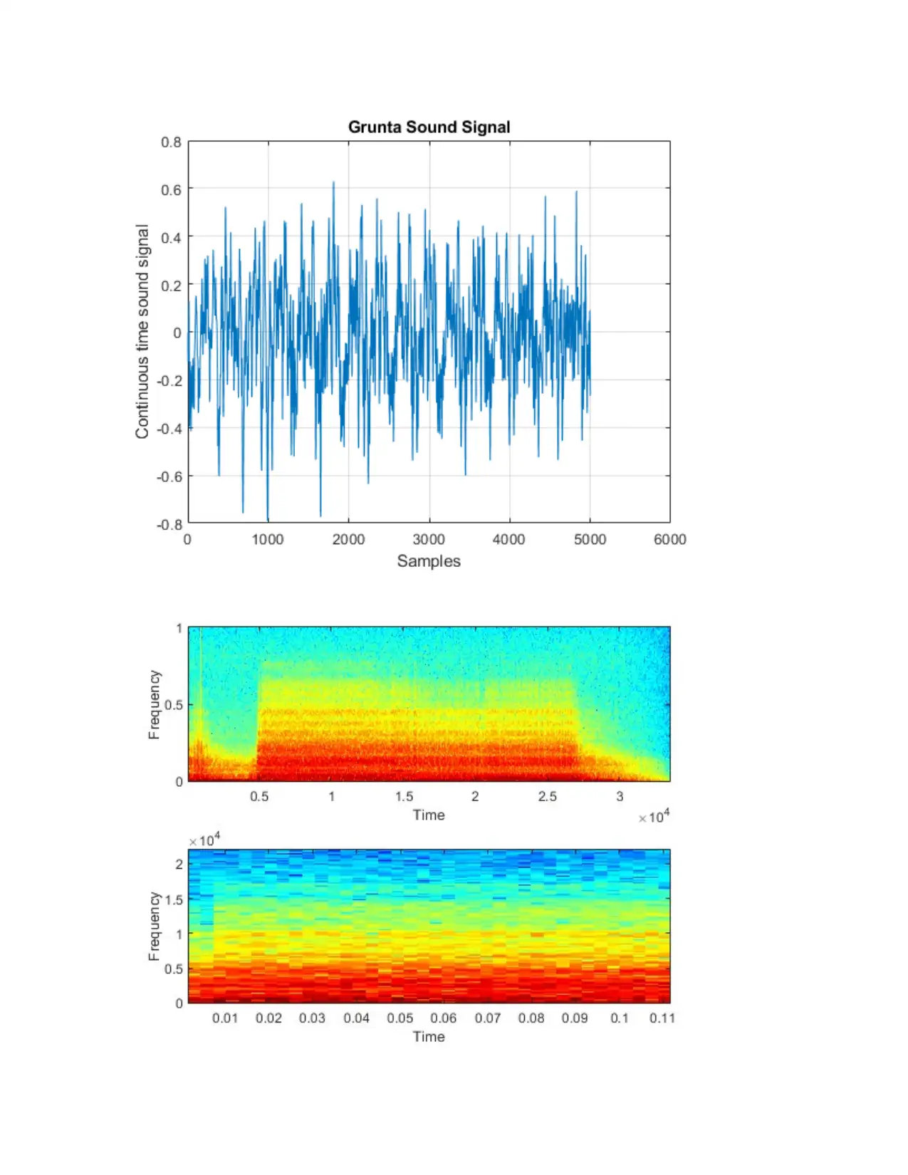
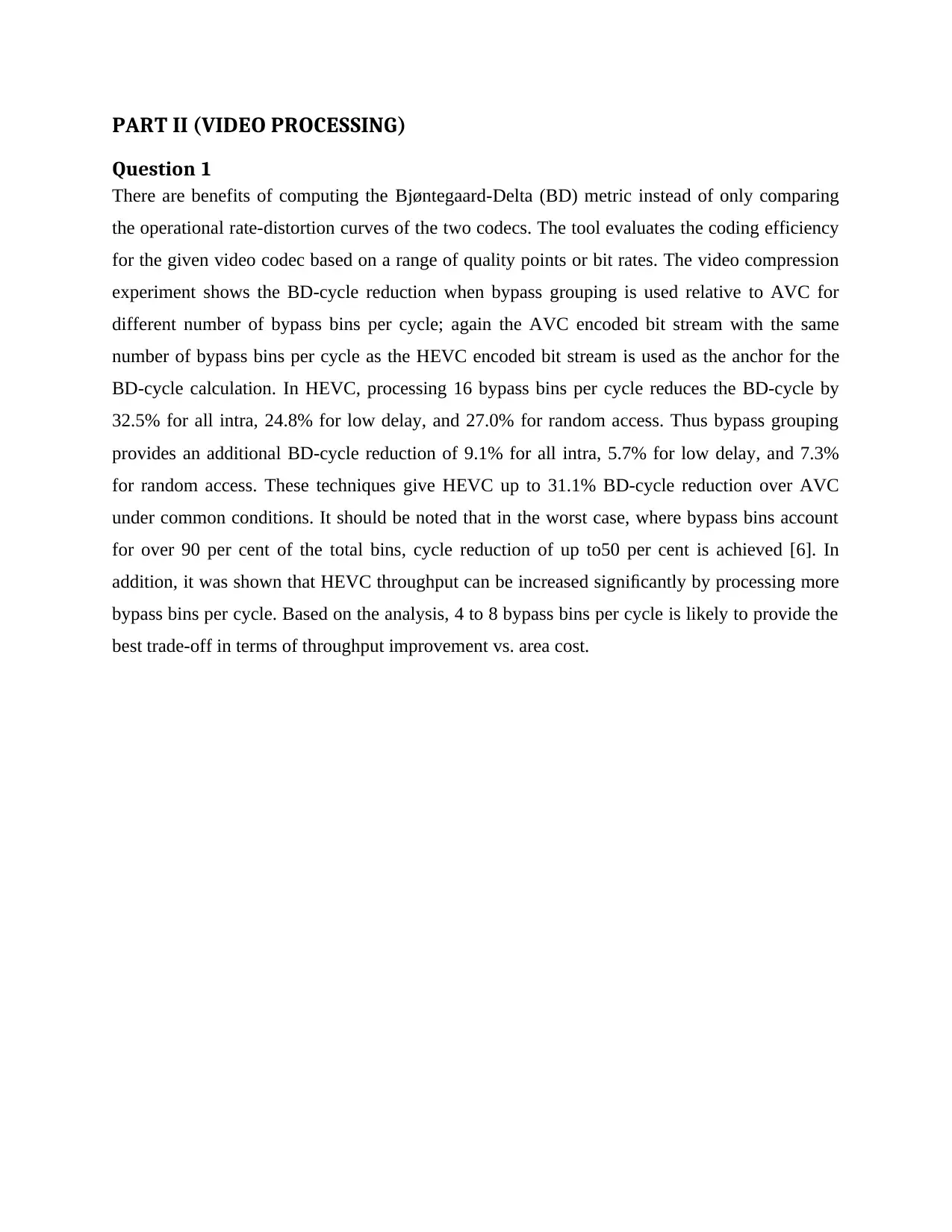
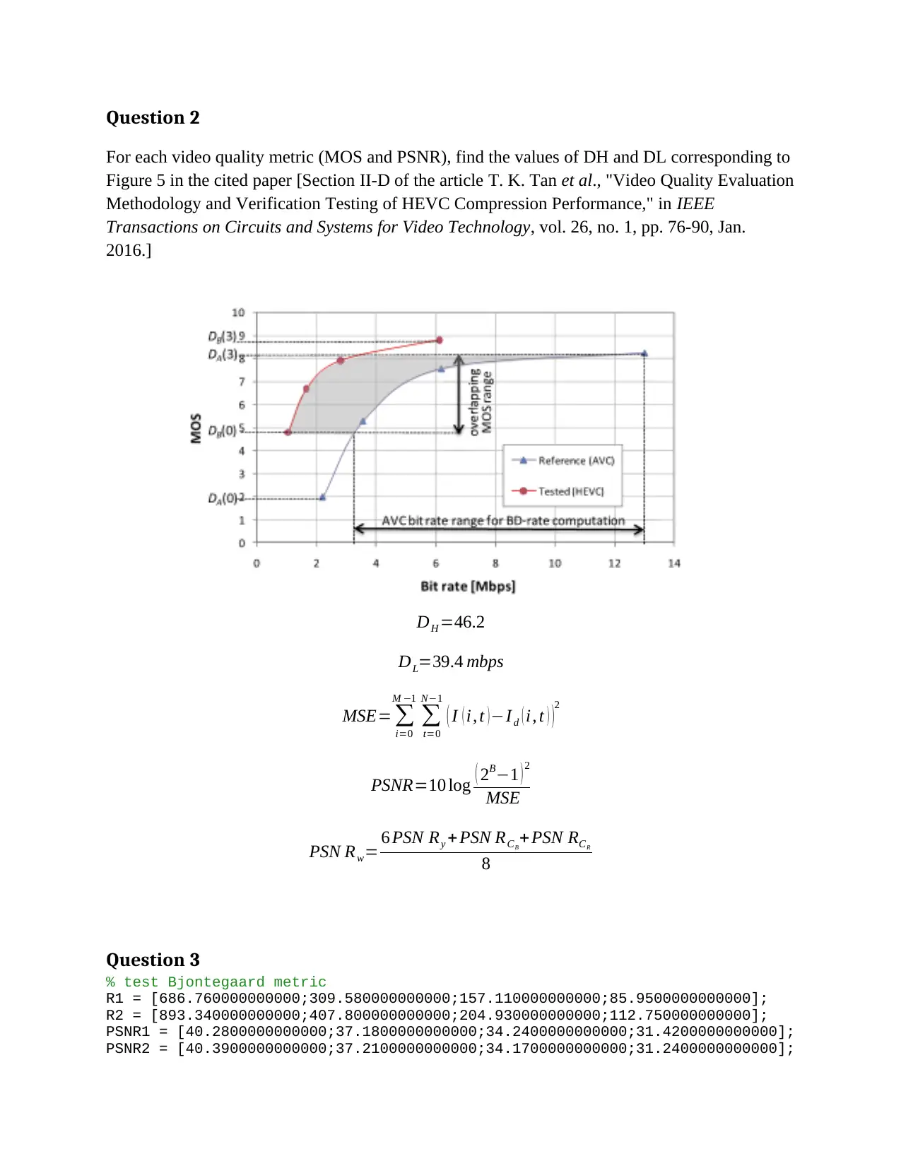
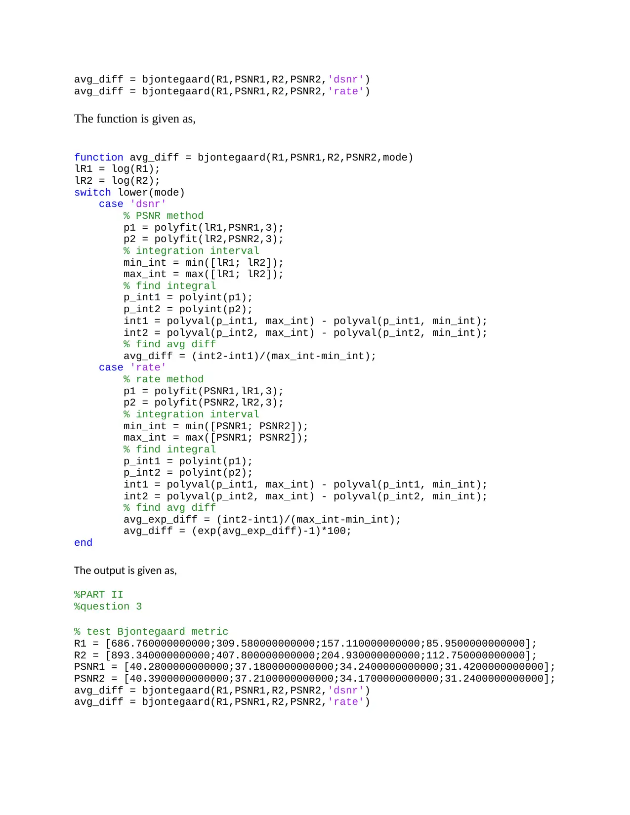
This report presents a detailed analysis of signal processing and video compression techniques, addressing the problems outlined in the ENGT5111 Digital Signal Processing assignment. The first part of the report focuses on filter design and signal analysis, specifically addressing ECG signal processing and the application of filters to remove muscle noise. It includes the design and implementation of a recursive filter suitable for ECG signals, along with a discussion on the output of the filters for a given input signal. The second part explores the spectrogram, its characteristics, and its use in analyzing audio signals, with an example using a WAV file. The report then transitions to video processing, examining the benefits of the Bjøntegaard-Delta (BD) metric for evaluating video codec efficiency and its application in HEVC compression. It further addresses the determination of video quality metrics and the computation of the BD metric using provided data. The report includes MATLAB code for signal analysis and video processing calculations, demonstrating practical application of the concepts discussed.

ENGT5111 Digital
Signal Processing
Signal Analysis and Video Compression
2018
Student Name
Student ID Number

PROBLEM 1
y ( n )= 1
21 (−2 x [ n ]+3 x [ n−1 ] +6 x [ n−2 ] + 7 x [ n−3 ]+6 x [ n−4 ]+3 x [ n−5 ]−2 x [ n−6 ] )
Section 1
An electrocardiogram (ECG) defines a time-varying signal that demonstrates the ionic
current flow which causes the cardiac fibers to contract and subsequently relax. The signals are
collected using a device that measures and records the electrical activity of the heart from
electrodes placed on specific points of a person’s skin. The signal is used by cardiologists to
detect heart related illnesses such as the coronary artery disease, the left ventricular hypertrophy,
kalemia, myocardial, valvular and congenial heart disease. The most common method uses 12
distinct points where the leads are placed. The ECG trace represents several electrical entities
such as the P wave, the QRS complex, and the T wave.
Some of the most common noises captured during the ECG recording are the baseline
wander, power line interference, and muscle noise. The ECG filter y(n) aims at removing the
noise without altering the desired information in the biomedical ECG signal recorded. The linear
phase filter maybe implemented as it avoids phase distortion that can alter various temporal
relationships in the cardiac cycle. Some filters are ineffective when small knots are recorded

whereas performing a polyfit() affects the heart rate outlook. This particular filter is a nonlinear
filter whose output is based on the input.
The ECG signal is recorded as a repetitive signal that uses ensemble averaging
techniques. The width functions especially for the low pass filter that have variable frequency
response, the width function is designed to reflect local signal attribute that show smooth
segments of the ECG. The ECG is filtered to remove errors. An ECG signal corrupted by muscle
noise which causes the low amplitude waveforms which are obstructed during the recording of
the ECG signal. It is quite difficult to remove it without affecting the ECG signal attributes since
it overlaps with the complex PQRST. It is not in any way linked to the narrow band filtering. The
muscle noise overlaps with actual ECG data recorded.
Section 2
Design and implementation of a recursive filter for the ECG signal
f =∑
m ,n
( f , ψm ,n ) ψm ,n
ϕ ( x
2 )=20.5
∑
n
h ( n ) ϕ ( x−n )
ψ ( x
2 )=20.5
∑
n
g ( n ) ϕ ( x−n )
d j+1( p)=∑
n
g ( n−2 p ) a j (n)
a j+1 ( p)=∑
n
h ( n−2 p ) aj ( n)
T =σ √ 2 log n

PRD=
√ ∑
n=0
N
( V ( n ) −V R ( n ) )
2
∑
n=0
N
V 2 ( n )
SNR=log10
∑
n=0
N
V R
2 ( n )
∑
n=0
N
S R
2 ( n )
It has shorter frequency response transition width despite having issues of system instability.
Section 3
Expression of the output of the two filters given the input signal is x [n]=cos(0.35 n)
y [ n ] = 1
21 (−2 x [ n ] +3 x [ n−1 ]+ 6 x [ n−2 ] +7 x [n−3 ] +3 x [ n−5 ]−2 x [ n−6 ] )
FreqS = 44.35; % Sampling
frequency
fcuts = [0.5 1.0 45 46]; % Frequency
Vector
mags = [0 1 0]; % Magnitude
(Defines Passbands & Stopbands)
devs = [0.05 0.01 0.05]; % Allowable
Deviations
[n,Wn,beta,ftype] = kaiserord(fcuts,mags,devs,FreqS);
n = n + rem(n,2);
hh = fir1(n,Wn,ftype,kaiser(n+1,beta),'scale');
figure(1)
freqz(hh, 1, 2^14, FreqS)

PROBLEM 2
Section 1
Spectrogram in acoustic signals
Acoustic signals capture human speech or any other form of sound. The acoustic signals
are recorded based on the articulation. Speech is dynamic as it is affected by the pitch, loudness,
quality and as a result it is transmitted at different frequencies over time. The speech filter varies
over time as the speech is articulated. The sound signal is represented using an amplitude and
time. The frequency response of the signal is obtained from the recorded continuous time signal.
There are several ways to analyze and review the acoustic signal. The amplitude spectrum
represents the amplitude and frequency albeit the time. The original form of the sound signal
representation is using the time waveform. It can also be represented as an amplitude spectrum.
The spectrogram combines the time, amplitude, and frequency attributes of a signal. All the
components are equally represented.
Good quality dynamic signal spectra are desired in real world applications. For instance,
one would want to hear a good voice on radio as opposed to a distorted speech of very poor
quality. The spectrogram is obtained when a sequence of spectra is stacked together in time and
the amplitude axis is compressed. The system plots frequency against time while the amplitude is

demonstrated using a line illustration on the two axes. The graph demonstrates the energy
content with black sections illustrating the highly concentrated regions with the highest
amplitude while white shows the least concentrated regions or the noise floor. Any region that is
represented between these extreme regions is the varying shades of grey. An acoustic signal is
analyzed using a sound spectrograph which produces the spectrogram as the output. The
spectrograph captures the dynamics of speech and may vary only in frequency, amplitude, and
time. There are two types of spectrograms such as wide-band spectrogram and the narrow-band
spectrogram. The wide band spectrogram has a short time spectrum calculation with damped
analysis filter while the narrow band spectrogram produces an analytic scheme that emphasizes
the change in the frequency of a signal. The spectrogram, therefore, represents how the
frequency content of a signal changes with time. The table below compares the two types of
signal spectrograms,
Wide-band spectrograms Narrow-band spectrograms
1. Bandwidth of the analyzing filter is
broad (300Hz)
1. It has a narrow bandwidth (45 Hz)
2. Compared to the spectrum envelopes 2. Compared to the amplitude spectra
3. 3.
Section 2
Using a wav file to analyze the sound and signal spectrum. The wav file used in this case is the
Grunta.wav file. The speech or audio signal is a sound amplitude that varies in time. The wav
file is a digital signal that is further analyzed using the signal spectrogram. The values can vary
continuously or take from a discrete set, the time and space and can also be continuous or
discrete. Using matlab signal to analyze the audio file,
Digital signal processing
%PART I
%problem 1
clear all
close all

%problem 2
[y,fs]=audioread('Grunta.wav');
sound(y,fs);
figure(1)
plot(y)
grid on
title('Grunta Sound Signal')
xlabel('Samples')
ylabel('Continuous time sound signal')
x=y(10000:15000)
figure(2)
plot(x)
grid on
title('Grunta Sound Signal')
xlabel('Samples')
ylabel('Continuous time sound signal')
%Sampling the speech spectrogram
figure(3)
subplot(2,1,1)
specgram(y)
subplot(2,1,2)
specgram(x,256,fs) %outputs the line spectra
%PART II

PART II (VIDEO PROCESSING)
Question 1
There are benefits of computing the Bjøntegaard-Delta (BD) metric instead of only comparing
the operational rate-distortion curves of the two codecs. The tool evaluates the coding efficiency
for the given video codec based on a range of quality points or bit rates. The video compression
experiment shows the BD-cycle reduction when bypass grouping is used relative to AVC for
different number of bypass bins per cycle; again the AVC encoded bit stream with the same
number of bypass bins per cycle as the HEVC encoded bit stream is used as the anchor for the
BD-cycle calculation. In HEVC, processing 16 bypass bins per cycle reduces the BD-cycle by
32.5% for all intra, 24.8% for low delay, and 27.0% for random access. Thus bypass grouping
provides an additional BD-cycle reduction of 9.1% for all intra, 5.7% for low delay, and 7.3%
for random access. These techniques give HEVC up to 31.1% BD-cycle reduction over AVC
under common conditions. It should be noted that in the worst case, where bypass bins account
for over 90 per cent of the total bins, cycle reduction of up to50 per cent is achieved [6]. In
addition, it was shown that HEVC throughput can be increased significantly by processing more
bypass bins per cycle. Based on the analysis, 4 to 8 bypass bins per cycle is likely to provide the
best trade-off in terms of throughput improvement vs. area cost.

Question 2
For each video quality metric (MOS and PSNR), find the values of DH and DL corresponding to
Figure 5 in the cited paper [Section II-D of the article T. K. Tan et al., "Video Quality Evaluation
Methodology and Verification Testing of HEVC Compression Performance," in IEEE
Transactions on Circuits and Systems for Video Technology, vol. 26, no. 1, pp. 76-90, Jan.
2016.]
DH =46.2
DL=39.4 mbps
MSE= ∑
i=0
M −1
∑
t=0
N−1
( I ( i, t )−I d ( i, t ) )2
PSNR=10 log ( 2B−1 ) 2
MSE
PSN Rw= 6 PSN Ry + PSN RCB
+ PSN RCR
8
Question 3
% test Bjontegaard metric
R1 = [686.760000000000;309.580000000000;157.110000000000;85.9500000000000];
R2 = [893.340000000000;407.800000000000;204.930000000000;112.750000000000];
PSNR1 = [40.2800000000000;37.1800000000000;34.2400000000000;31.4200000000000];
PSNR2 = [40.3900000000000;37.2100000000000;34.1700000000000;31.2400000000000];

avg_diff = bjontegaard(R1,PSNR1,R2,PSNR2,'dsnr')
avg_diff = bjontegaard(R1,PSNR1,R2,PSNR2,'rate')
The function is given as,
function avg_diff = bjontegaard(R1,PSNR1,R2,PSNR2,mode)
lR1 = log(R1);
lR2 = log(R2);
switch lower(mode)
case 'dsnr'
% PSNR method
p1 = polyfit(lR1,PSNR1,3);
p2 = polyfit(lR2,PSNR2,3);
% integration interval
min_int = min([lR1; lR2]);
max_int = max([lR1; lR2]);
% find integral
p_int1 = polyint(p1);
p_int2 = polyint(p2);
int1 = polyval(p_int1, max_int) - polyval(p_int1, min_int);
int2 = polyval(p_int2, max_int) - polyval(p_int2, min_int);
% find avg diff
avg_diff = (int2-int1)/(max_int-min_int);
case 'rate'
% rate method
p1 = polyfit(PSNR1,lR1,3);
p2 = polyfit(PSNR2,lR2,3);
% integration interval
min_int = min([PSNR1; PSNR2]);
max_int = max([PSNR1; PSNR2]);
% find integral
p_int1 = polyint(p1);
p_int2 = polyint(p2);
int1 = polyval(p_int1, max_int) - polyval(p_int1, min_int);
int2 = polyval(p_int2, max_int) - polyval(p_int2, min_int);
% find avg diff
avg_exp_diff = (int2-int1)/(max_int-min_int);
avg_diff = (exp(avg_exp_diff)-1)*100;
end
The output is given as,
%PART II
%question 3
% test Bjontegaard metric
R1 = [686.760000000000;309.580000000000;157.110000000000;85.9500000000000];
R2 = [893.340000000000;407.800000000000;204.930000000000;112.750000000000];
PSNR1 = [40.2800000000000;37.1800000000000;34.2400000000000;31.4200000000000];
PSNR2 = [40.3900000000000;37.2100000000000;34.1700000000000;31.2400000000000];
avg_diff = bjontegaard(R1,PSNR1,R2,PSNR2,'dsnr')
avg_diff = bjontegaard(R1,PSNR1,R2,PSNR2,'rate')

∆ Roverall ≈ 10
1
D H −D L
∫
DL
D H
[ ^rB ( D ) − ^r A ( D ) ] dD−1
avgdiff =−1.1922
avgdiff =31.4244
REFERENCES
[1]. Zhang Li-Bao. Region of interest image coding using iwt and partial bit plane block shift
for network applications. In Computer and Information Technology, 2005.CIT 2005. The
Fifth International Conference on, pages 624 – 628, sept. 2005
[2]. P. Artameeyanant. Image watermarking using adaptive tabu search. In ICCAS-SICE,
2009, pages 1941 –1944, aug. 2009.
[3]. Lijie Liu and Guoliang Fan. A new jpeg2000 region-of-interest image coding method:
partial significant bit planes shift. Signal Processing Letters, IEEE, 10(2):35 – 38, feb
2003.
[4]. Strang G. and Strela V., “Short Wavelets and Matrix Dilation Equations,” IEEE
Transactions Signal Processing, vol. 43, pp. 108-115, 2005.
[5]. Vetterli M. and Kovacevic J., Wavelets and Sub band Coding, Englewood Cliffs,
Prentice Hall, 1995, http /cm.bell-labs.com/ who/ jelena/Book/ home.html.
[6]. Wiegand T., Sullivan G., Bjontegaard G., and Luthra A., “Overview of the H.264 / AVC
Video Coding Standard,” IEEE Transactions on Circuits System Video Technology, pp.
243-250, 2003.
[7]. Wonkookim and Chung C., “On Preconditioning Multi wavelet System for Image
Compression,” International Journal of Wavelets Multi resolution and Information
Processing, vol. 1, no. 1, pp. 51-74, 2003.
[8]. K. R. Namuduri and V. N. Ramaswamy, “Feature preserving image compression,” in
Pattern Recognition Letters, vol. 24, no. 15, pp. 2767-2776, Nov. 2003.
[9]. B. E. Usevitch, “A Tutorial on Modern Lossy Wavelet Image Compression: Foundations
of JPEG 2000,” in IEEE Signal processing Magazine, vol. 18, no. 5, pp. 22-35, Sep. 2001
[10]. C. A. Gonzales, “DCT Coding of Motion Sequences Including Arithmetic Coder,”
ISO/IEC JCT1/SC2/WP8, MPEG 89/187, MPEG 89/187, 2009.