Signal Processing: AM Modulation Techniques with MATLAB Analysis

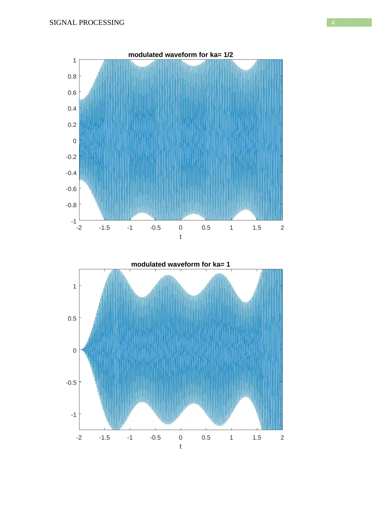
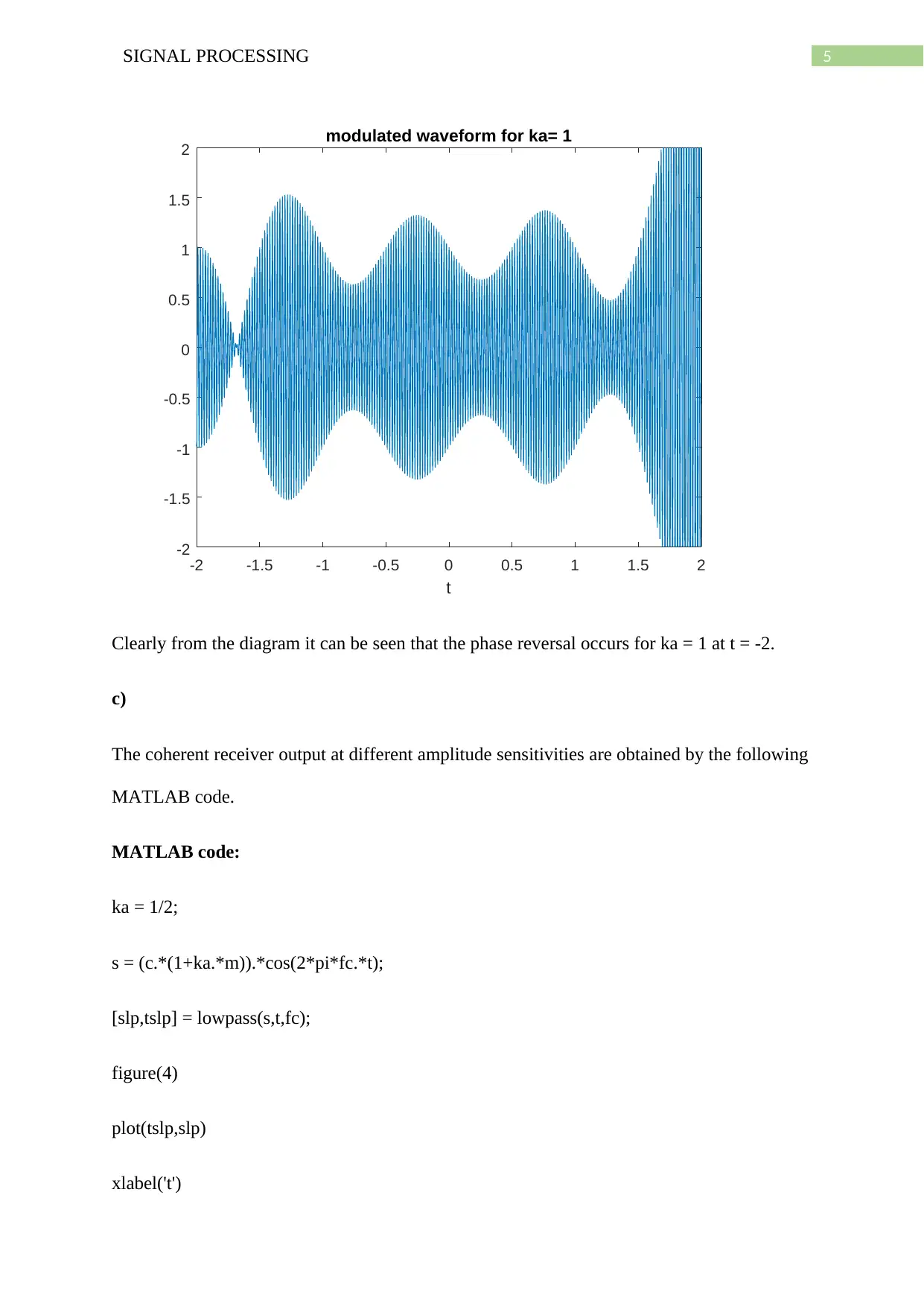
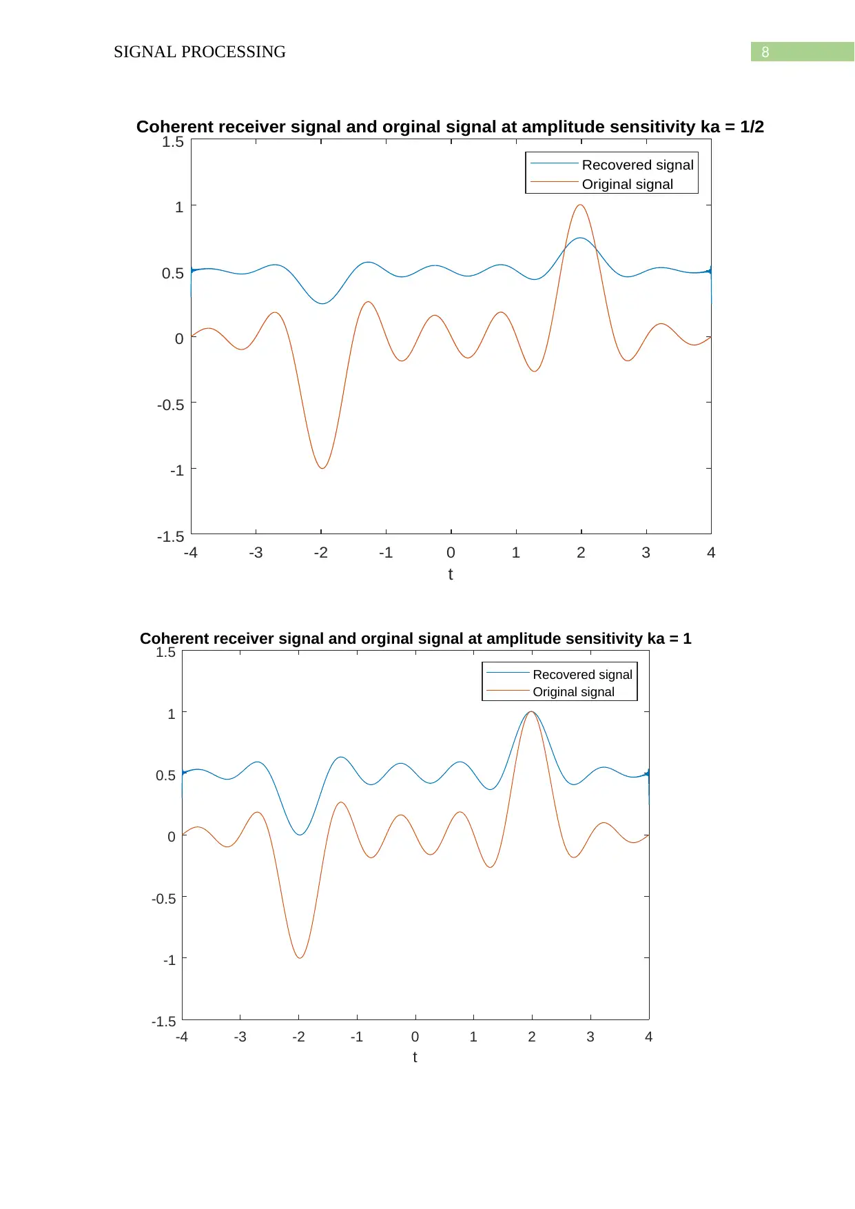
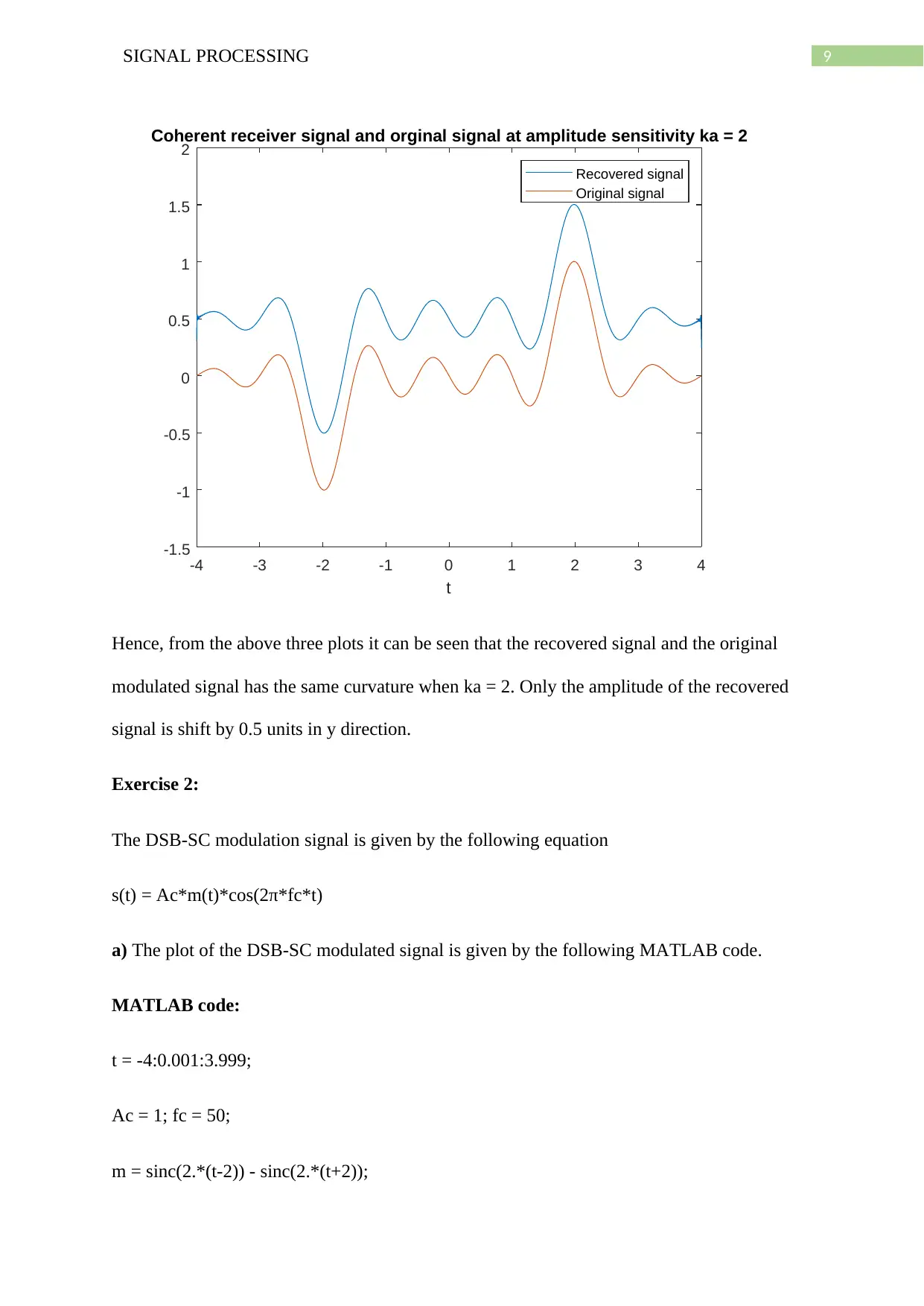
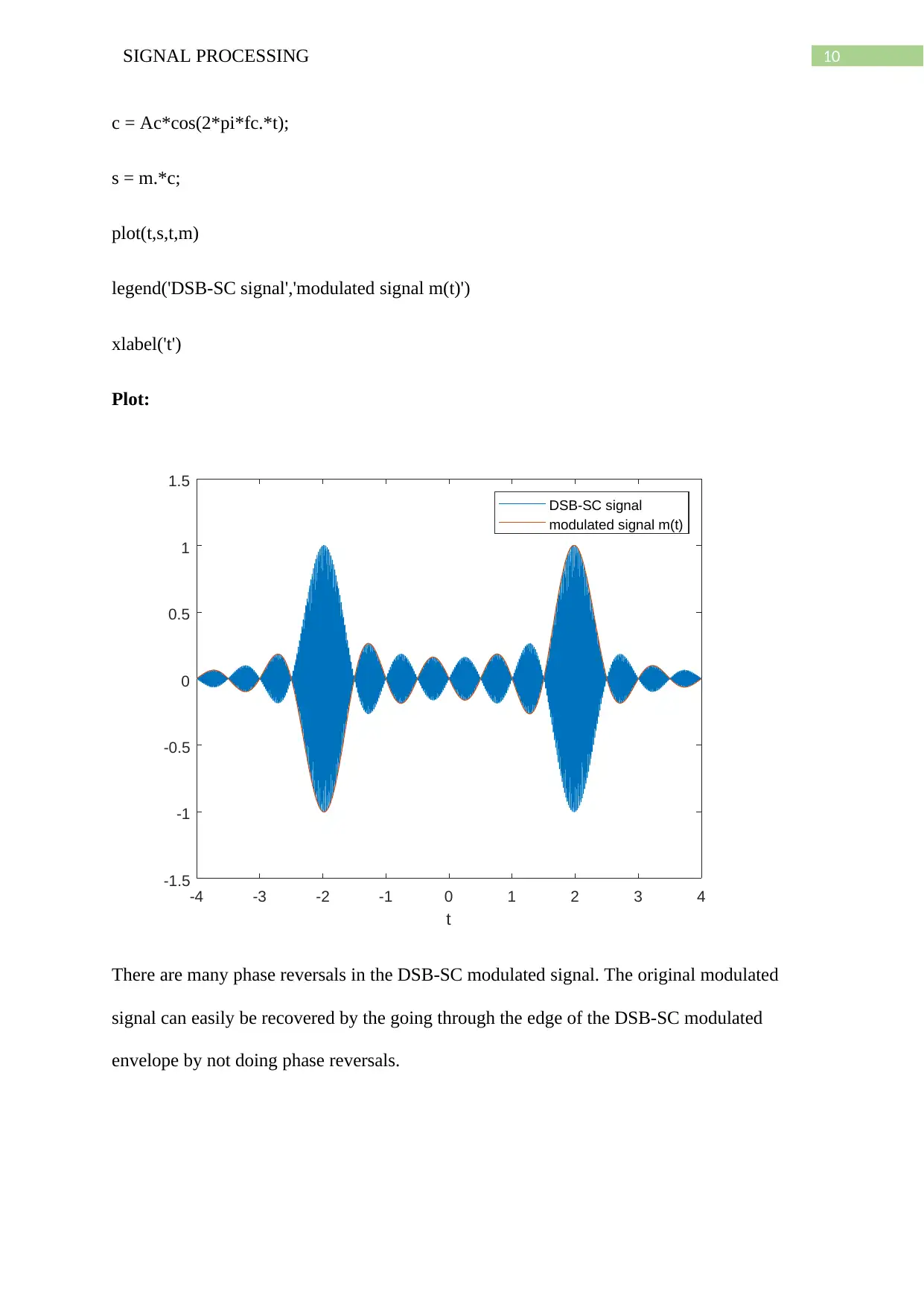
This assignment delves into Amplitude Modulation (AM) techniques, specifically Double-Sideband (DSB) and Suppressed-Sideband (SSB) methods, using MATLAB for analysis and implementation. The first part focuses on standard AM, examining modulated waveforms for varying amplitude sensitivities and coherent receiver outputs. It identifies phase reversals and signal recovery characteristics. The second part explores DSB-SC modulation, analyzing its waveforms and coherent receiver output with and without frequency deviations. The third part investigates suppressed-sideband AM, including DSB-SC, USSB, and LSSB modulations, plotting information signals, Hilbert transforms, and amplitude spectra. It also recovers the original signal from LSSB modulation. Finally, the assignment examines the amplitude spectrum of USSB and LSSB signals with frequency variations and demodulates the USSB signal. The MATLAB code is provided for each exercise, along with corresponding plots and analysis.

Running head: SIGNAL PROCESSING
SIGNAL PROCESSING
Name of the Student
Name of the University
Author Note

1SIGNAL PROCESSING
Part I: Double-SideBand AM
Exercise 1: Standard AM
Given, modulated signal is
s(t) = Ac[1 + ka*m(t)]cos(2*π*fc*t)
The information bearing signal is
m(t) = sinc(2(t-2)) – sinc(2(t+2))
The carrier signal is c(t) = Ac*cos(2πfct), Ac = 1 is the amplitude of carrier and fc = 50 Hz is
the carrier frequency.
a) The plot of signal m(t) and carrier c(t) is given below.
MATLAB code:
t = -4:0.001:3.999;
Ac = 1; fc = 50;
m = sinc(2.*(t-2)) - sinc(2.*(t+2));
c = Ac*cos(2*pi*fc.*t);
plot(t,m,'b-',t,c,'r-')
title('m(t) and c(t)')
legend('m(t)','c(t)')
xlabel('t')
ylabel('information signal and carrier signal amplitude')
zoom(2)

2SIGNAL PROCESSING
Plot:
-2 -1.5 -1 -0.5 0 0.5 1 1.5 2
t
-0.6
-0.4
-0.2
0
0.2
0.4
0.6
information signal and carrier signal amplitude
m(t) and c(t)
m(t)
c(t)
b) The modulated waveforms for different values of Ac are obtained by the following
MATLAB codes.
MATLAB code:
ka = 1/2;
s = c.*(1+ka.*m);
figure(1)
plot(t,s)
xlabel('t')
title('modulated waveform for ka= 1/2')

3SIGNAL PROCESSING
zoom(2)
ka = 1;
s = c.*(1+ka.*m);
figure(2)
plot(t,s)
xlabel('t')
title('modulated waveform for ka= 1')
zoom(2)
ka = 2;
s = c.*(1+ka.*m);
figure(3)
plot(t,s)
xlabel('t')
title('modulated waveform for ka= 1')
zoom(2)
Plots:

4SIGNAL PROCESSING
-2 -1.5 -1 -0.5 0 0.5 1 1.5 2
t
-1
-0.8
-0.6
-0.4
-0.2
0
0.2
0.4
0.6
0.8
1 modulated waveform for ka= 1/2
-2 -1.5 -1 -0.5 0 0.5 1 1.5 2
t
-1
-0.5
0
0.5
1
modulated waveform for ka= 1

5SIGNAL PROCESSING
-2 -1.5 -1 -0.5 0 0.5 1 1.5 2
t
-2
-1.5
-1
-0.5
0
0.5
1
1.5
2 modulated waveform for ka= 1
Clearly from the diagram it can be seen that the phase reversal occurs for ka = 1 at t = -2.
c)
The coherent receiver output at different amplitude sensitivities are obtained by the following
MATLAB code.
MATLAB code:
ka = 1/2;
s = (c.*(1+ka.*m)).*cos(2*pi*fc.*t);
[slp,tslp] = lowpass(s,t,fc);
figure(4)
plot(tslp,slp)
xlabel('t')

6SIGNAL PROCESSING
hold on
plot(t,m)
legend('Recovered signal','Original signal')
title('Coherent receiver signal and orginal signal at amplitude sensitivity ka = 1/2')
ka = 1;
s = (c.*(1+ka.*m)).*cos(2*pi*fc.*t);
[slp,tslp] = lowpass(s,t,fc);
figure(5)
plot(tslp,slp)
xlabel('t')
hold on
plot(t,m)
legend('Recovered signal','Original signal')
title('Coherent receiver signal and orginal signal at amplitude sensitivity ka = 1')
ka = 2;
s = (c.*(1+ka.*m)).*cos(2*pi*fc.*t);
[slp,tslp] = lowpass(s,t,fc);
figure(6)

7SIGNAL PROCESSING
plot(tslp,slp)
xlabel('t')
hold on
plot(t,m)
legend('Recovered signal','Original signal')
title('Coherent receiver signal and orginal signal at amplitude sensitivity ka = 2')
function [slp,tslp] = lowpass(s,ts,fcut)
B = fcut;
h = 2*B*sinc(2*B*ts);
N = length(ts);
Dty = ts(2)- ts(1);
tslp = ts;
slp = conv(h,s)*Dty;
slp = slp((N/2) + 1:(N/2) + N);
end
Plots:

8SIGNAL PROCESSING
-4 -3 -2 -1 0 1 2 3 4
t
-1.5
-1
-0.5
0
0.5
1
1.5
Coherent receiver signal and orginal signal at amplitude sensitivity ka = 1/2
Recovered signal
Original signal
-4 -3 -2 -1 0 1 2 3 4
t
-1.5
-1
-0.5
0
0.5
1
1.5
Coherent receiver signal and orginal signal at amplitude sensitivity ka = 1
Recovered signal
Original signal

9SIGNAL PROCESSING
-4 -3 -2 -1 0 1 2 3 4
t
-1.5
-1
-0.5
0
0.5
1
1.5
2
Coherent receiver signal and orginal signal at amplitude sensitivity ka = 2
Recovered signal
Original signal
Hence, from the above three plots it can be seen that the recovered signal and the original
modulated signal has the same curvature when ka = 2. Only the amplitude of the recovered
signal is shift by 0.5 units in y direction.
Exercise 2:
The DSB-SC modulation signal is given by the following equation
s(t) = Ac*m(t)*cos(2π*fc*t)
a) The plot of the DSB-SC modulated signal is given by the following MATLAB code.
MATLAB code:
t = -4:0.001:3.999;
Ac = 1; fc = 50;
m = sinc(2.*(t-2)) - sinc(2.*(t+2));

10SIGNAL PROCESSING
c = Ac*cos(2*pi*fc.*t);
s = m.*c;
plot(t,s,t,m)
legend('DSB-SC signal','modulated signal m(t)')
xlabel('t')
Plot:
-4 -3 -2 -1 0 1 2 3 4
t
-1.5
-1
-0.5
0
0.5
1
1.5
DSB-SC signal
modulated signal m(t)
There are many phase reversals in the DSB-SC modulated signal. The original modulated
signal can easily be recovered by the going through the edge of the DSB-SC modulated
envelope by not doing phase reversals.

11SIGNAL PROCESSING
b) Now, the output of the coherent receiver where the DSB-SC modulated signal is
multiplied by a carrier wave of 50 Hz and then passed through a low pass filter of cut-off
frequency of 50 Hz is obtained by the following MATLAB code as given below.
MATLAB code:
t = -4:0.001:3.999;
s = (m.*c).*cos(2*pi*(fc).*t);
[slp,tslp] = lowpass(s,t,fc);
figure(2)
plot(tslp,slp)
xlabel('t')
hold on
plot(t,m)
legend('Output signal of coherent receiver','Original DSB-SC modulated signal')
title('Coherent receiver signal and orginal modulated signal')
function [slp,tslp] = lowpass(s,ts,fcut)
B = fcut;
h = 2*B*sinc(2*B*ts);
N = length(ts);
Dty = ts(2)- ts(1);
tslp = ts;