Signals and Systems Assignment: Fourier Transform & Analysis

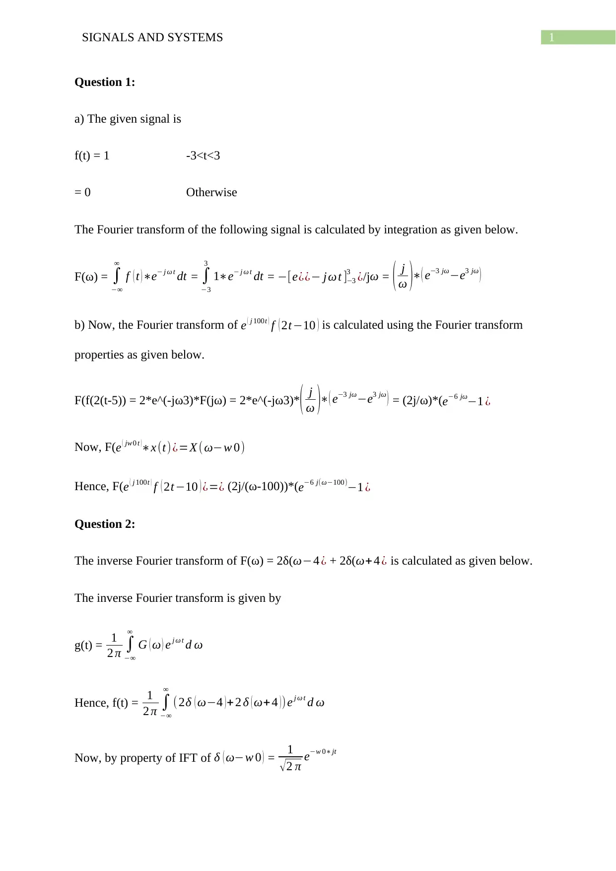
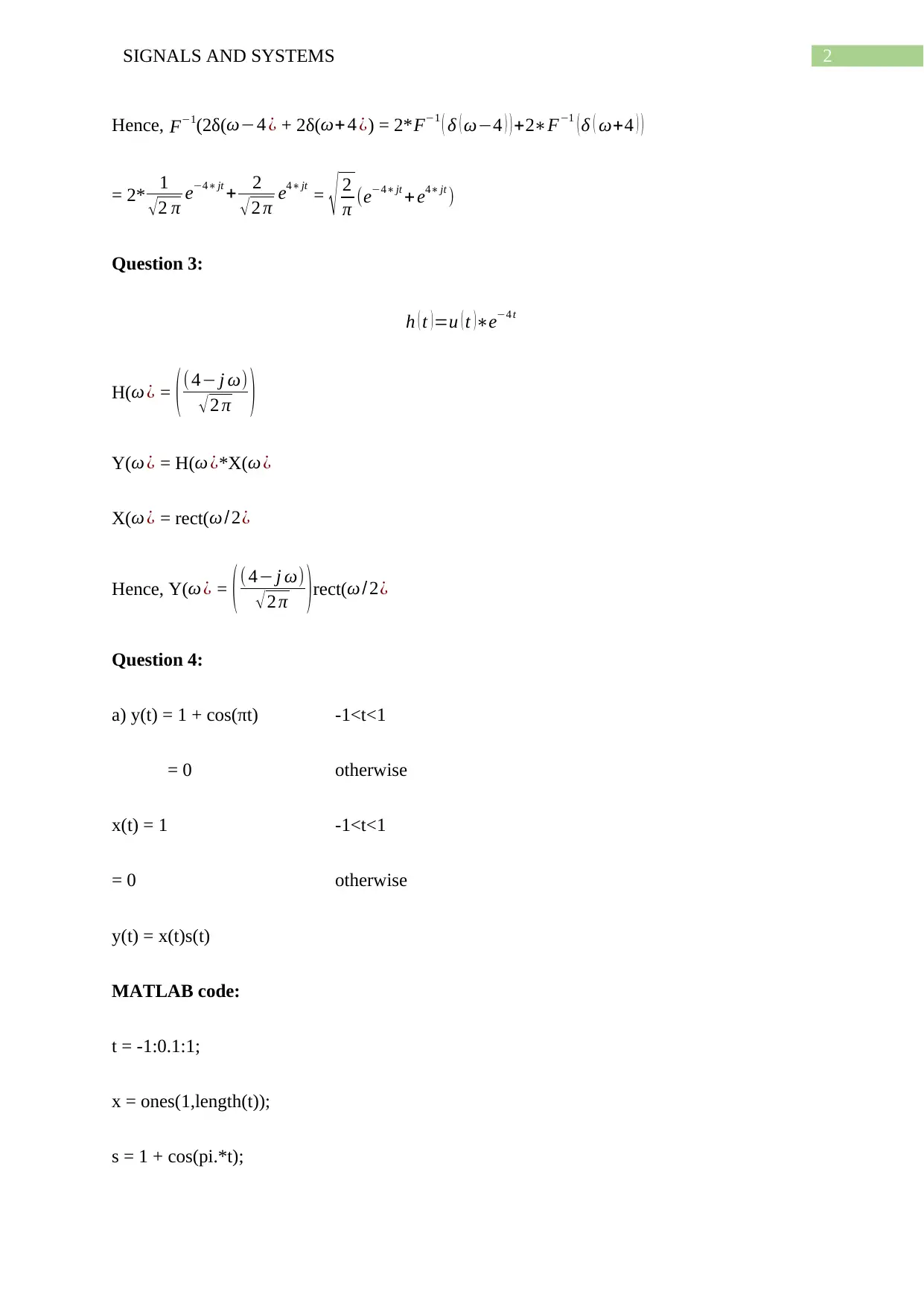
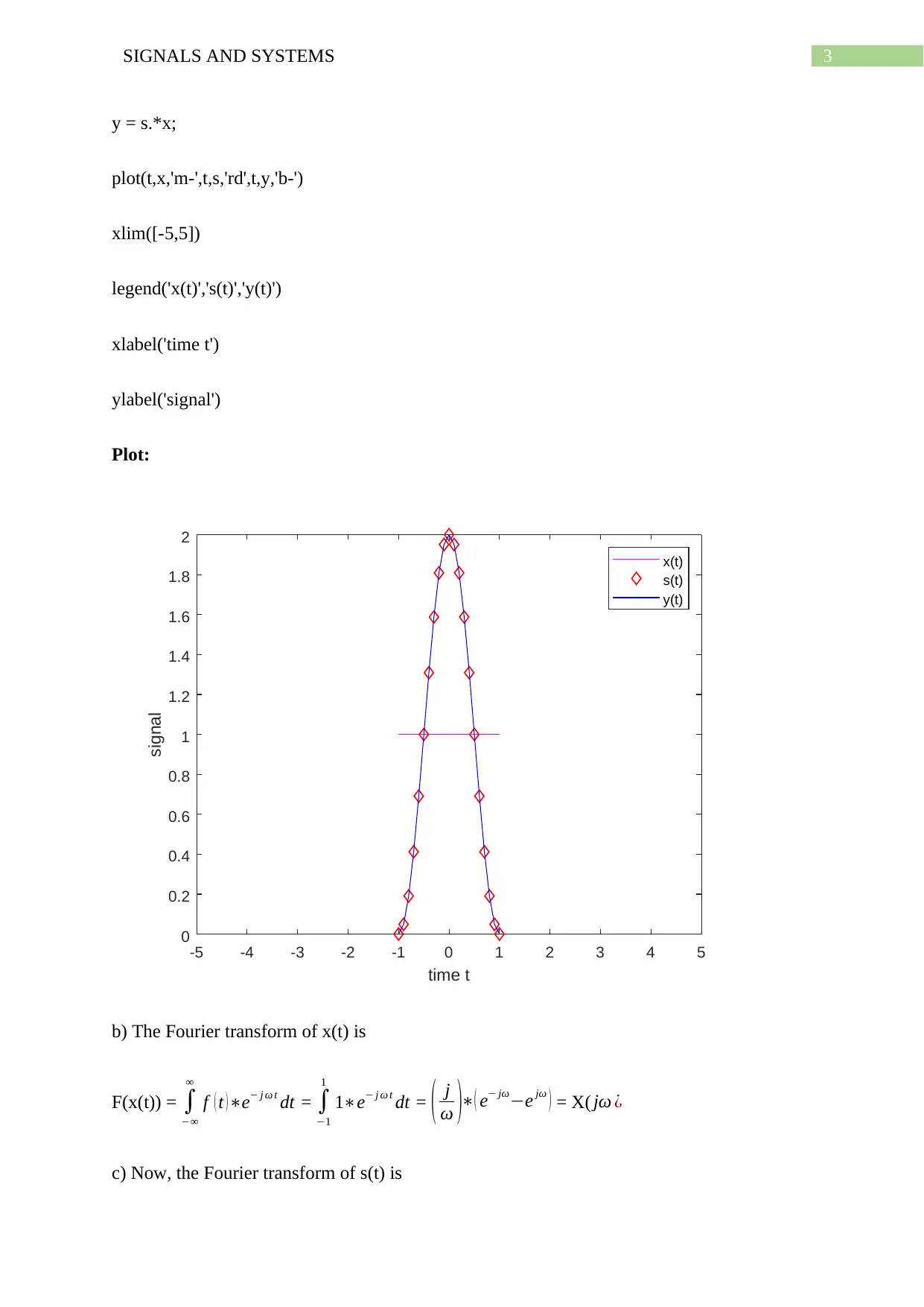
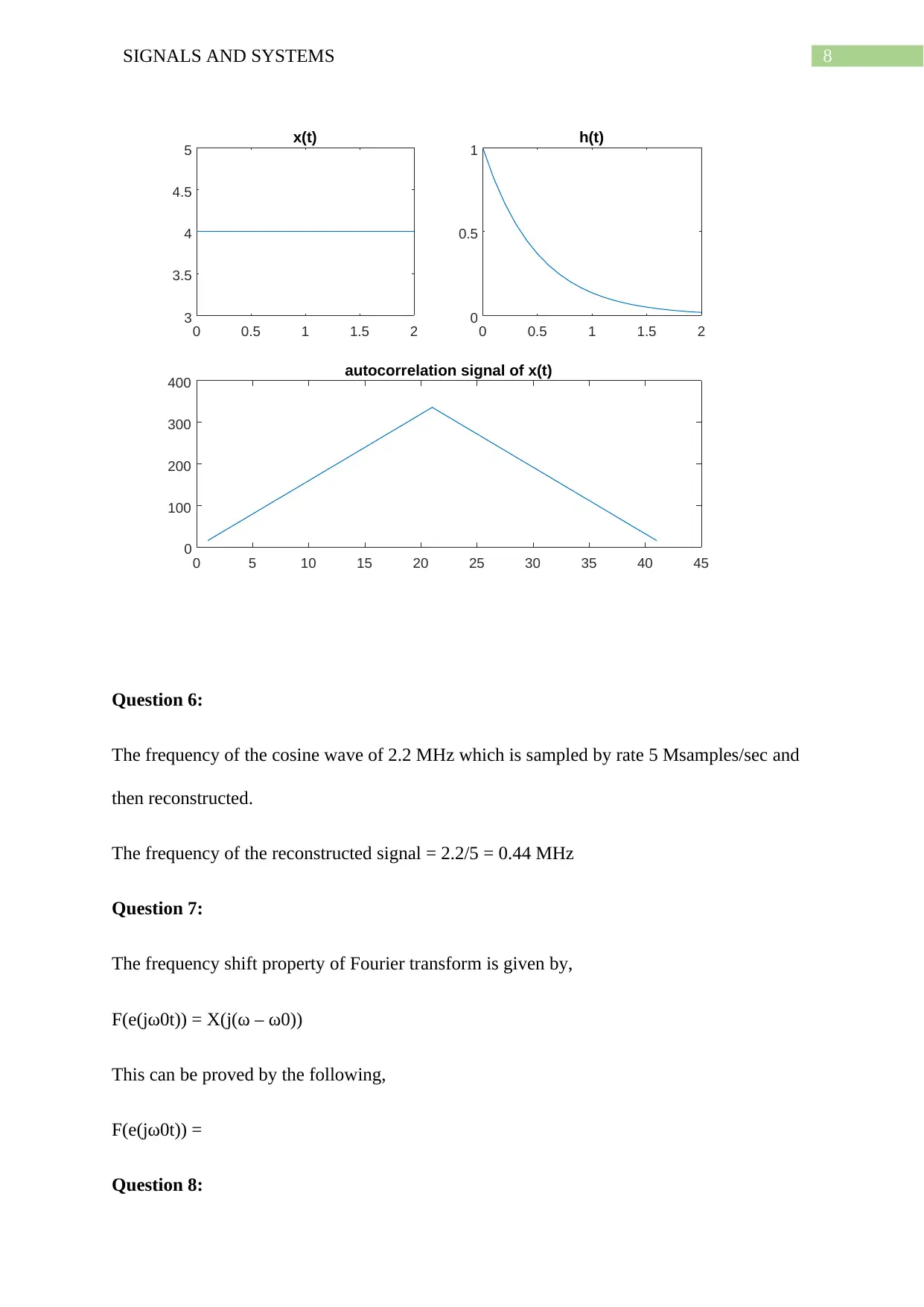
This document presents a comprehensive solution to a Signals and Systems assignment. The solution includes detailed calculations and explanations for several problems. Question 1 involves calculating the Fourier transform of a given signal and then applying Fourier transform properties. Question 2 focuses on finding the inverse Fourier transform of a given frequency-domain function. Question 3 analyzes an LTI system with a given impulse response and input signal, determining the Fourier transform of the output. Question 4 delves into the raised cosine pulse, requiring students to analyze its construction, Fourier transforms, and product in time domain. Question 5 explores energy spectral density, autocorrelation, and Parseval's theorem for a given signal, with MATLAB code for plotting and verification. Question 6 addresses the reconstruction of a sampled signal. The remaining questions touch on frequency shift properties, Fourier transform properties and the concept of real and imaginary components of a signal. The assignment covers a range of core concepts, including Fourier analysis, system analysis, and MATLAB implementation, providing a complete and insightful solution to the assignment.

0SIGNALS AND SYSTEMS
SIGNALS AND SYSTEMS
Name of the Student
Name of the University
Author Note

1SIGNALS AND SYSTEMS
Question 1:
a) The given signal is
f(t) = 1 -3<t<3
= 0 Otherwise
The Fourier transform of the following signal is calculated by integration as given below.
F(ω) = ∫
−∞
∞
f ( t ) ∗e− j ω t dt = ∫
−3
3
1∗e− j ω t dt = −[e¿¿− jω t ]−3
3 ¿/jω = ( j
ω )∗( e−3 jω−e3 jω )
b) Now, the Fourier transform of e ( j 100t ) f ( 2t−10 ) is calculated using the Fourier transform
properties as given below.
F(f(2(t-5)) = 2*e^(-jω3)*F(jω) = 2*e^(-jω3)*( j
ω )∗( e−3 jω−e3 jω ) = (2j/ω)*(e−6 jω−1 ¿
Now, F(e ( jw0 t )∗x (t)¿=X ( ω−w 0)
Hence, F(e ( j 100t ) f ( 2t−10 ) ¿=¿ (2j/(ω-100))*(e−6 j(ω−100)−1 ¿
Question 2:
The inverse Fourier transform of F(ω) = 2δ(ω−4 ¿ + 2δ(ω+ 4 ¿ is calculated as given below.
The inverse Fourier transform is given by
g(t) = 1
2 π ∫
−∞
∞
G ( ω ) e j ω t d ω
Hence, f(t) = 1
2 π ∫
−∞
∞
( 2δ ( ω−4 ) + 2 δ ( ω+ 4 ) )e j ω t d ω
Now, by property of IFT of δ ( ω−w 0 ) = 1
√2 π e−w 0∗ jt

2SIGNALS AND SYSTEMS
Hence, F−1(2δ(ω−4 ¿ + 2δ(ω+ 4 ¿) = 2*F−1 ( δ ( ω−4 ) ) +2∗F−1 ( δ ( ω+4 ) )
= 2* 1
√2 π e−4∗ jt + 2
√ 2 π e4∗ jt
= √ 2
π (e−4∗ jt + e4∗ jt )
Question 3:
h ( t )=u ( t )∗e−4 t
H(ω ¿ = (( 4− j ω)
√2 π )
Y(ω ¿ = H(ω ¿*X( ω ¿
X(ω ¿ = rect( ω /2¿
Hence, Y(ω ¿ = ( ( 4− j ω)
√ 2 π )rect(ω / 2¿
Question 4:
a) y(t) = 1 + cos(πt) -1<t<1
= 0 otherwise
x(t) = 1 -1<t<1
= 0 otherwise
y(t) = x(t)s(t)
MATLAB code:
t = -1:0.1:1;
x = ones(1,length(t));
s = 1 + cos(pi.*t);

3SIGNALS AND SYSTEMS
y = s.*x;
plot(t,x,'m-',t,s,'rd',t,y,'b-')
xlim([-5,5])
legend('x(t)','s(t)','y(t)')
xlabel('time t')
ylabel('signal')
Plot:
-5 -4 -3 -2 -1 0 1 2 3 4 5
time t
0
0.2
0.4
0.6
0.8
1
1.2
1.4
1.6
1.8
2
signal
x(t)
s(t)
y(t)
b) The Fourier transform of x(t) is
F(x(t)) = ∫
−∞
∞
f ( t )∗e− j ω t dt = ∫
−1
1
1∗e− j ω t dt = ( j
ω )∗( e− jω−e jω ) = X( jω ¿
c) Now, the Fourier transform of s(t) is

4SIGNALS AND SYSTEMS
F(s(t)) = F(1 + cos(πt)) = F(1) + F(cos(πt)) = ( j
ω )∗( e− jω−e jω ) − jω exp (− jω ) ( exp ( 2 jω )−1 )
j2 ω2 +π 2
¿ ( π 2 )∗exp ( − jω ) ( exp ( 2 j ω ) −1 )
jω ( j2 ω2 +π 2 ) = S( jω ¿
d) Now, by the property of Fourier transform product in time domain = convolution in
frequency domain.
Hence, by formula
F(y(t)) = F(x(t)s(t)) = X( jω ¿∗S ( jω) = ( 1
2 π )∗∫
−1
1
X ( j ω' ) S ( j ( ω−ω' ) ) d ω'
Now, computing the integral we get the same result as
Y(ω ¿ = ( π 2 )∗exp ( − j ω ) ( exp ( 2 j ω ) −1 )
jω ( j2 ω2 +π 2 )
Question 5:
a) Given signal,
x(t) = 4, 0< t <2
= 0 Otherwise
Energy spectral density E = ∫
0
2
[ x ( t ) ]
2
dt = ∫
0
2
[ 4 ] 2
dt = 16*2 = 32.
b) The auto-correlation function of the continuous-time signal is given by,
Rff(τ) = ∫
0
2
x ( t+ τ ) x (t )' d t= ∫
0
2
2∗2 d t= ∫
0
2
4 d t= 4(2-0)= 8.
c) The Parseval’s theorem of the signal is given by,

5SIGNALS AND SYSTEMS
Power P = ∫
−∞
∞
|x ( t )|
2
dt= 1
2 π ∫
−∞
∞
| X ( ω )|
2
dω = ∫
−∞
∞
| X ( 2 πf )|
2
df
d) The energy spectral density of the output signal is given by,
ESD = |H ( ω )|2
∗|X ( ω )|2
Where, H(ω) = F(h(t)) = 1/(2 + jω)
X(ω) = 4(1-exp(-j2ω))/(jω)
|X(ω)|^2 = (16/ω^2)
Hence, ESD = (16/(ω^2)(4 + ω^2))
e) The total energy of output signal is given by,
E = ∫
0
2
( 16
( ω2 ) ( 4+ω2 ) ) d ω
f) The MATLAB code for plot of x(t), h(t), autocorrelation of x(t) and spectral density of
input x(t) and y(t) is given below.
MATLAB code:
t = 0:0.1:2;
x = repmat(4,1,length(t));
h = exp(-2.*t);
y = h.*x;
autocorrx = xcorr(x);
inputpsd = dspdata.psd(x);
figure(1)

6SIGNALS AND SYSTEMS
subplot(2,1,1)
plot(inputpsd)
title('plot of input PSD')
outputpsd = dspdata.psd(y);
subplot(2,1,2)
plot(outputpsd)
title('plot of output PSD')
figure(2)
subplot(2,2,1)
plot(t,x)
title('x(t)')
subplot(2,2,2)
plot(t,h)
title('h(t)')
subplot(2,2,[3 4])
plot(autocorrx)
title('autocorrelation signal of x(t)')
energyx = sum(x.^2)
energyy = sum(y.^2)
Output:

7SIGNALS AND SYSTEMS
energyx =
336
energyy =
48.5210
0 0.1 0.2 0.3 0.4 0.5 0.6 0.7 0.8 0.9 1
Normalized Frequency ( rad/sample)
5
5.5
6
6.5
7
Power/frequency (dB/(rad/sample))
plot of input PSD
0 0.1 0.2 0.3 0.4 0.5 0.6 0.7 0.8 0.9 1
Normalized Frequency ( rad/sample)
-10
-5
0
5
10
Power/frequency (dB/(rad/sample))
plot of output PSD

8SIGNALS AND SYSTEMS
0 0.5 1 1.5 2
3
3.5
4
4.5
5 x(t)
0 0.5 1 1.5 2
0
0.5
1 h(t)
0 5 10 15 20 25 30 35 40 45
0
100
200
300
400 autocorrelation signal of x(t)
Question 6:
The frequency of the cosine wave of 2.2 MHz which is sampled by rate 5 Msamples/sec and
then reconstructed.
The frequency of the reconstructed signal = 2.2/5 = 0.44 MHz
Question 7:
The frequency shift property of Fourier transform is given by,
F(e(jω0t)) = X(j(ω – ω0))
This can be proved by the following,
F(e(jω0t)) =
Question 8:

9SIGNALS AND SYSTEMS
Given that x(t) is purely imaginary
From the Fourier transform property it is known that
If, F(x(t)) = X(jω) then F(x*(t)) = X*(-jω)
Now, if x(t) = ja, where, a is any constant
F(ja) = aX(ω) and F(-ja) = (-a)X*(-ω)
Hence, X(ω) = - X*(-ω)
Question 9:
h(t) = Real(g(t)*exp(jω0t))
H(ω) = F(h(t))
Re(z) = (z + z’)/2
Let, z = a + jb, z’ = a – jb
Re(z) = a
Hence, F(Re(z)) = a*delta(t)

10SIGNALS AND SYSTEMS