Signals and Systems Assignment 1: Analysis, Solutions and MATLAB Plots

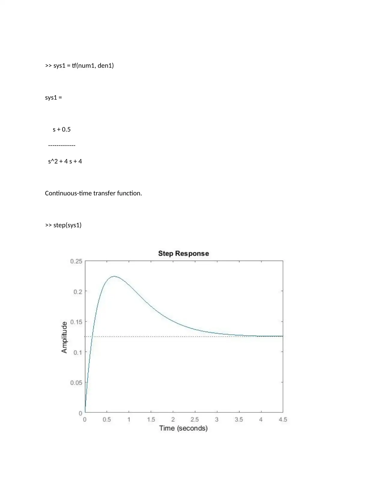
This document presents a comprehensive solution to a Signals and Systems assignment. It begins by analyzing a system's characteristic equation, roots, and modes, and then proceeds to determine the transfer function. The solution includes calculations for the zero-input response, impulse response, and zero-state output using convolution and MATLAB. The document further explores the total system response, natural and forced responses, and provides MATLAB code for plotting impulse, step, and frequency responses. Finally, it examines the step response of an LTI system, the frequency response, and the output for a given input signal. It also includes the analysis of a signal in both the time and frequency domains, alongside the effects of a low-pass filter.

a. Find the characteristic equation, characteristic roots and characteristic modes of
this system:
Characteristic equation:
d2y(t)/dt2 + 4.dy(t)/d(t) +4y(t) = dx(t)/dt + 0.5 x(t)
Taking Laplace transfome:
L{d2y(t)/dt2} + 4L {dy(t)/d(t)} + 4L {y(t)} = L{dx(t)/dt} + 0.5L {x(t)}
Transfer Function = Laplace transform of output / Laplace Transform of input
Initial conditions sets to be zero:
y(0) = 0
x(0) = 0
H(s) = Y(s)/X(s) = (s+0.5)/ (s2 + 4s + 4)
Characteristics Roots:
(s +0.5) = 0
S= -0.5
Poles:
s+0.5 = 0,
s= -0.5,
Zeroes:
(s2 + 4s + 4) = 0
Taking the partial fraction:
s2 + (2 +2) s+ 4=0
s2 + 2s+2s+ 4=0
(s+2) (s+2) = 0
s = -2,-2.
Characteristic modes:

If the number of poles are less than the number of zeros i.e. Z > P then the value of transfer
function becomes infinity. Hence it shows that there are poles at infinity and the number of such
poles is (Z-P)
Poles < Zeroes
b. Comment on the stability of the system.
H(s) = Y(s)/X(s) = (s+0.5)/ (s2 + 4s + 4)
Poles:
s+0.5 = 0,
s= -0.5
Zeroes:
(s+2) (s+2) = 0
s = -2,-2.
When the poles of the system are located in the left-half plane (LHP) and the system is not
improper, the system is shown to be stable.

c. Find y0(t), the zero-input component of the response For t ≥ 0, if the initial
conditions are y(0) = 3 and y (0) = −4.
Characteristic equation:
d2y(t)/dt2 + 4.dy(t)/d(t) +4y(t) = dx(t)/dt + 0.5 x(t)
d2y(t)/dt2 + 4.dy(t)/d(t) +4y(t) = 0
λ2 + 4 λ + 4 = 0
(λ +2) (λ +2) = 0
λ = -2,-2
yh (t) = C1 e-2t + C2 e-2t

y0(t) = 3, 3 = C1 +C2
y’0(t) = dy0(t)/dt
y’0(t) = -2 e-2t - 2 e-2t
y’0(t) = -4, -4= -2C1 - 2C2
4 = 2 C1 + 2C2
C1 = 1
C2 = 4
Y0 (t) = e-2t + 4 e-2t
d. Mathematically derive an expression for (t)ℎ , the impulse response of the system.
H(s) = (s+0.5)/ (s2 + 4s + 4)
h(t) = L-1H(s)
h(t) = L-1 {(s+0.5)/ (s2 + 4s + 4)}
h(t) = L-1 {(s+0.5)/ (s+2)2}
(s+0.5)/ (s+2)2 = a 0
( s+2) + a 1
( s+2)2
For the denominator root:
a0 = 1
a1 = -1.5
h(t) = L-1{ 1
(s+2) - 1.5
( s+2) 2}
Use the linearity property of inverse Laplace transform:

L-1{ 1
( s+2 ) } = e-2t
L-1{ 1.5
(s+2) 2} = 1.5 e-2t.t
h(t) = e-2t - 1.5 e-2t.t
(e) Using the convolution tables and the result of part (d), find the zero-state output for the
system given the input
x(t) = e-3t . u(t)
MATLAB coding for zero input:
>> t=linspace(0,30);
>> xzi=1*exp(-3*t)
plot(t,xzi,'m')
title('x_{zi}(t) vs. t'); xlabel('t, (s)'); ylabel('x_{zi}(t), (m)'); axis([0 30 -5 10]);

h(t) = e-2t - 1.5 e-2t.t
MATLAB coding for zero state:
>> t=linspace(0,30);
xzi=1*exp(-2*t)-1.5*exp(-2*t)
plot(t,xzi,'m')
title('x_{zi}(t) vs. t'); xlabel('t, (s)'); ylabel('x_{zi}(t), (m)'); axis([0 30 -5 10]);
Y(t) = x(t) * h(t)
Y(t) = e-3t . u(t). e-2t - 1.5 e-2t.t
.
:

f. What is the total system response based on the conditions and input specified above?
Total system response:
Y(t) = Yn (t) + Yf(t)
Y(t) = e-2t + 4 e-2t +0.833 e-2t + 1.25 e-2t - 2.5 e-3t
Y(t) = 7.083 e-2t - 2.5 e-3t
g. What is the natural response and what is the forced response of this system?
Natural Response:
Characteristic equation:
d2y(t)/dt2 + 4.dy(t)/d(t) +4y(t) = dx(t)/dt + 0.5 x(t)
d2y(t)/dt2 + 4.dy(t)/d(t) +4y(t) = 0
λ2 + 4 λ + 4 = 0
(λ +2) (λ +2) = 0
λ = -2,-2
yh (t) = C1 e-2t + C2 e-2t
y0(t) = 3, 3 = C1 +C2
y’0(t) = dy0(t)/dt
y’0(t) = -2 e-2t - 2 e-2t
y’0(t) = -4, -4= -2C1 - 2C2
4 = 2 C1 + 2C2
C1 = 1
C2 = 4

Natural Response:
Yn (t) = e-2t + 4 e-2t
Forced response:
Given Input is x(t) = e-3t
Yp(t) = k. e-3t
d Yp(t) / dt = k.(-3.e-3t)
d2 Yp(t) / dt2 = k.(9.e-3t)
k(9.e-3t) – 12.k.e-3t + 4k.e-3t = 3.e-3t +0.5e-3t
k=-2.5
Forced response:
Yp (t) = -2.5 e-3t
Yf(t) = yh(t) + yp(t)
Yf(t) = C1 e-2t + C2 e-2t - 2.5 e-3t
Y(0) = C1 + C2 -2.5
dY(0) / dt = -2 C1 - 2 C2 +7.5
C1=0.833, C2 = 1.25
Yf(t) = 0.833 e-2t + 1.25 e-2t - 2.5 e-3t

(h) Using Matlab, plot the impulse and step responses and frequency response (magnitude
and phase) of this system directly from the differential equation.
d2y(t)/dt2 + 4.dy(t)/d(t) +4y(t) = dx(t)/dt + 0.5 x(t)
L{d2y(t)/dt2} + 4L {dy(t)/d(t)} + 4L {y(t)} = L{dx(t)/dt} + 0.5L {x(t)}
Initial conditions to be zero:
y(0) = 0
x(0) = 0
H(s) = (s+0.5)/ (s2 + 4s + 4)
MATLAB CODING:
Frequency response (magnitude and phase)
>> bode(sys)
bode(sys1,sys2,...,sysN)
bode(sys1,LineSpec1,...,sysN,LineSpecN)
bode(___,w)
[mag,phase,wout] = bode(sys)
[mag,phase,wout] = bode(sys,w)
[mag,phase,wout,sdmag,sdphase] = bode(sys,w)
Undefined function or variable 'sys'.
>> H = tf([1 0.5],[1 4 4]);
>> bode(H)

Step Response MATLAB Coding:
>> num1=[1 0.5]
num1 =
1.0000 0.5000
>> den1= [1 4 4]
den1 =
1 4 4

>> sys1 = tf(num1, den1)
sys1 =
s + 0.5
-------------
s^2 + 4 s + 4
Continuous-time transfer function.
>> step(sys1)

Impulse Response MATLAB Coding:
>> h=impz([1 0.5],[1 4 4])
h =
1.0e+06 *
0.0000
-0.0000
0.0000
-0.0000
0.0001
-0.0002
0.0004
-0.0008
0.0018
-0.0040
0.0087
-0.0189
0.0410
-0.0881
0.1884
-0.4014
0.8520