SIT718 Real World Analytics Assessment Task 4: Problem Solving Project

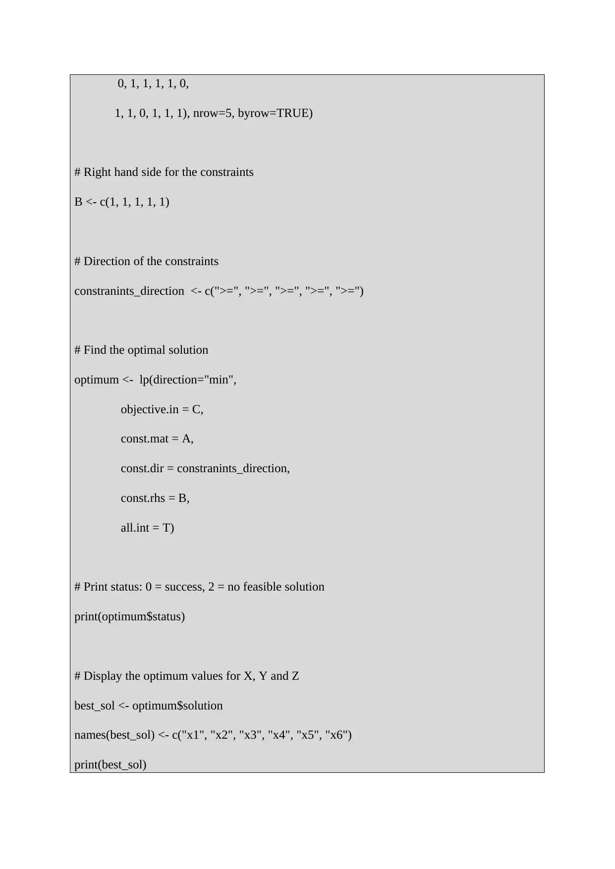
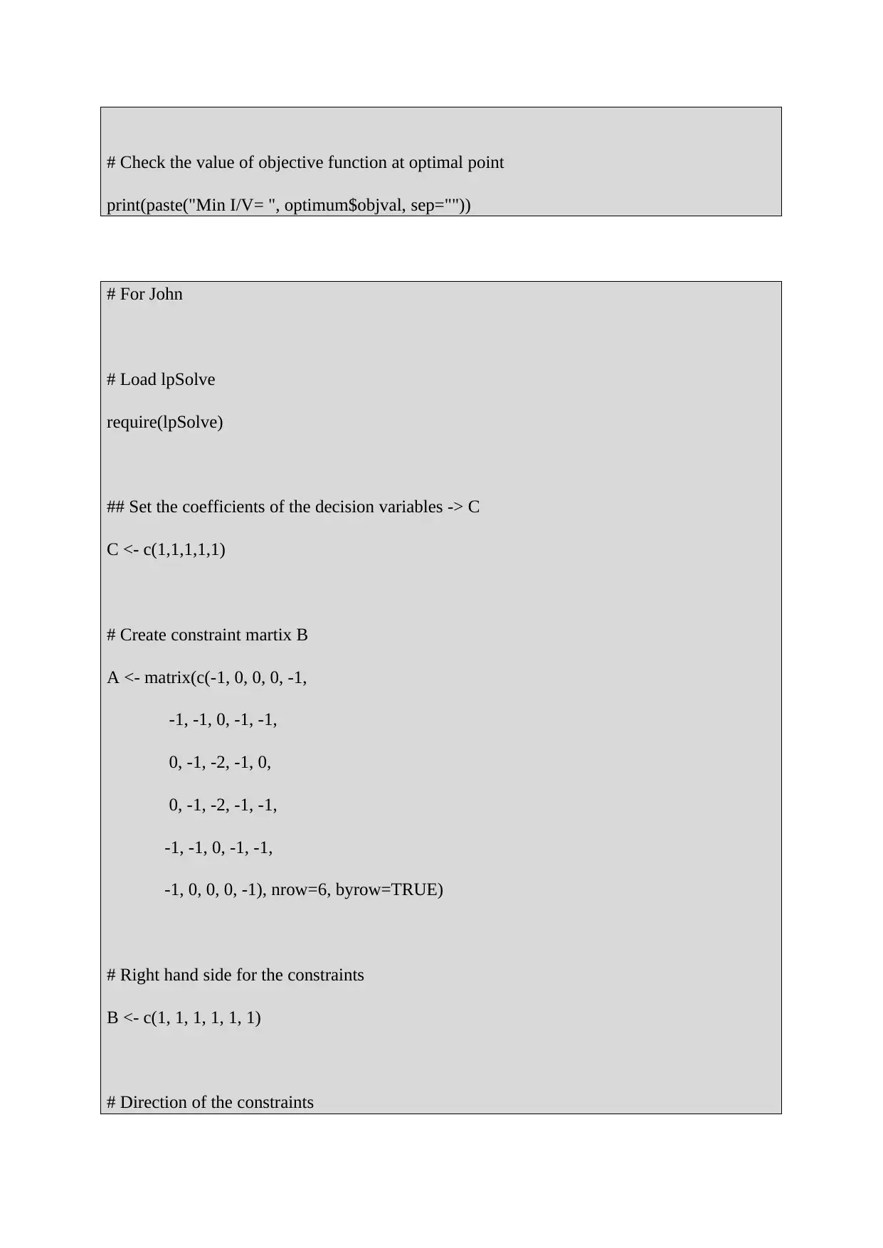
This document presents a comprehensive solution to SIT718 Real World Analytics Assessment Task 4, focusing on problem-solving using linear programming and game theory. The assignment includes three main questions. Question 1 explores linear programming (LP) by justifying its use, formulating an LP model for a manufacturing scenario, solving it graphically, and performing sensitivity analysis. Question 2 formulates an LP problem and solves it using R code, demonstrating computational problem-solving skills. Question 3 delves into game theory, specifically a two-player zero-sum game, involving payoff matrices, saddle points, and the formulation of linear programming models for both players. The solution includes R code implementations for solving the game and determining optimal strategies. The document also provides references to relevant academic literature.

SIT718 Real World Analytics
Assessment Task 4: Problem solving task 3
Name of the Student
Name of the University
Author Note

Table of Contents
Question 1:.................................................................................................................................3
Part [a] Justification behind using LP....................................................................................3
Part [b] Formulation of LP.....................................................................................................3
Part [c] Solving LP using graphical method...........................................................................4
Part [d] Sensitivity Analysis...................................................................................................5
Question 2:.................................................................................................................................5
Part [a] Formulation of LP problem:......................................................................................5
Part [b] Solving LP using R:..................................................................................................6
Question 3:.................................................................................................................................9
Part [a] Two players zero sum game......................................................................................9
Part [b] Payoff Matrix............................................................................................................9
Part [c] Saddle point...............................................................................................................9
Part [d] Linear programming model.......................................................................................9
Part [e] R code......................................................................................................................10
Part [f] Solution of the game................................................................................................13
Reference..................................................................................................................................15

Question 1:
Part [a] Justification behind using LP
While decision making, there are several tool or process available to come to a meaningful
conclusion. However, use of linear programming is considered as one of the best choice.
Taken for example, in this case, the manufacturing unit has limited labour hours as well as
raw materials. Now, given those consideration, if they want to maximize their revenue, use of
LP will be a helpful solution because:
1] It will allow to combine all resources and give us alternatives to opt;
2] It will show the best possible solution;
Part [b] Formulation of LP
Let us consider X is the number of unit of Dresses to be produced and Y is the number of unit
of Coats to be produced.
Hence, the profit the manufacturing unit will earn is
8X + 15Y
Therefore, the objective function will be
Max 8X + 15Y
Now the cutting constraint will be
25X + 12Y <= 12000
Sewing constraint will be
25X + 55Y <= 24960
The packaging constraint will be
15X + 15Y <= 6720
And the demand for dresses will be
X >= 120
And
Y >= 0

Part [c] Solving LP using graphical method
In order to solve this LP using graphical method, the first step is to consider all the in-
equalities as equality. Considering these, we have the graph as mentioned below:
The red line is 25x+12y=12000 … (1)
The green line is 25x+55y=24960 … (2)
The blue line is 15x+15y=6720 … (3)
And the sky blue line is x = 120 … (4)
Now applying the inequalities, we have the feasible region as shown below:

Now, the intersection point of (1) and (2) [A] is (335, 301)
Intersection point of (1) and (4) [B] is (120, 399)
Intersection point of (3) and (4) [C] is (120, 328)
The intersection point of (3) with X axis [D] is (448, 0)
And the intersection point of (1) with X axis [E] is (480, 0)
Now, at A, the objective function value is 7195
at B, the objective function value is 6945
at C, the objective function value is 5880
at D, the objective function value is 3584
at E, the objective function value is 3840
hence, the maximum profit the manufacturing unit can earn is $7195 and for that they have to
produce 335 units of Dresses and 301 unit of Coats.
Part [d] Sensitivity Analysis
In order to find out a range for the profit ($) of a dress that can be changed without affecting
the optimum solution obtained above, we have to check the slope of objective function. In
this specific case, the tangent point, which is the intersection point of (1) and (2) attained
maximum profit. Hence, it can be said that there is only one point and hence, instead of
range, the X value will be 335 only.
Question 2:
Part [a] Formulation of LP problem:
Let X, Y and Z denotes number of boxes of cereals A, B and C respectively to be produced.
As per given information, the total revenue from these three types of cereals will be:
2.60X + 2.30Y + 3.20Z
Now, the production cost of each type of cereals are given per ton. Hence, the production cost
for desired number of boxes will be:
(4.20/500)X + (2.60/500)Y + (3.00/500)Z

Also raw material costs are given per ton. Hence, the total raw material costs for desired
number of boxes will be:
(100/500)*(0.80X + 0.60Y + 0.45Z) + (90/500)*(0.10X + 0.25Y + 0.15Z) +
(110/500)*(0.05X + 0.05Y + 0.10Z) + (200/500)*(0.05X + 0.10Y + 0.30Z)
Hence, the total cost will be:
4.20/500)X + (2.60/500)Y + (3.00/500)Z + (100/500)*(0.80X + 0.60Y + 0.45Z) +
(90/500)*(0.10X + 0.25Y + 0.15Z) + (110/500)*(0.05X + 0.05Y + 0.10Z) +
(200/500)*(0.05X + 0.10Y + 0.30Z)
= 0.2075X + 0.2212Y + 0.2650Z
Hence, the total profit will be:
2.60X + 2.30Y + 3.20Z – (0.2075X + 0.2212Y + 0.2650Z)
=2.3925X + 2.0788Y + 2.935Z
Therefore, the objective function will be
Max 2.3925X + 2.0788Y + 2.935Z
Now the constraints are given as
X >= 1000
Y >= 800
Z >= 750
And
0.80X + 0.60Y + 0.45Z <= 10000
0.10X + 0.25Y + 0.15Z <= 5000
0.05X + 0.05Y + 0.10Z <= 2000
0.05X + 0.10Y + 0.30Z <= 2000
Part [b] Solving LP using R:
R code:
#install lpSolve

install.packages("lpSolve")
# Load lpSolve
require(lpSolve)
## Set the coefficients of the decision variables -> C
C <- c(2.3925, 2.0788, 2.935)
# Create constraint martix B
A <- matrix(c(1, 0, 0,
0, 1, 0,
0, 0, 1,
0.80, 0.60, 0.45,
0.10, 0.25, 0.15,
0.05, 0.05, 0.10,
0.05, 0.10, 0.30), nrow=7, byrow=TRUE)
# Right hand side for the constraints
B <- c(1000, 800, 750, 10000, 5000, 2000, 2000)
# Direction of the constraints
constranints_direction <- c(">=", ">=", ">=", "<=", "<=", "<=", "<=")
# Find the optimal solution
optimum <- lp(direction="max",

objective.in = C,
const.mat = A,
const.dir = constranints_direction,
const.rhs = B,
all.int = T)
# Print status: 0 = success, 2 = no feasible solution
print(optimum$status)
# Display the optimum values for X, Y and Z
best_sol <- optimum$solution
names(best_sol) <- c("X", "Y", "Z")
print(best_sol)
# Check the value of objective function at optimal point
print(paste("Total Profit: ", optimum$objval, sep=""))
R output:

Question 3:
Part [a] Two players zero sum game
A two-player game is called a zero-sum game if the sum of the two payoff matrices is zero.
The payoff to one player is always made by the other player (no externalities). In this case as
the sum of two payoff matrices is zero, we can say that this game is a two person zero sum
game.
Part [b] Payoff Matrix
Payoff score John
(Alice,
John) (P1, P2) (4,0) (3,1) (2,2) (1,3) (0,4)
Alice
(5,0) (1,-1) (0,0) (0,0) (0,0) (1,-1)
(4,1) (1,-1) (1,-1) (0,0) (1,-1) (1,-1)
(3,2) (0,0) (1,-1) (2,-2) (1,-1) (0,0)
(2,3) (0,0) (1,-1) (2,-2) (1,-1) (1,-1)
(1,4) (1,-1) (1,-1) (0,0) (1,-1) (1,-1)
(0,5) (1,-1) (0,0) (0,0) (0,0) (1,-1)
Part [c] Saddle point
Saddle point in game theory refers to a value of a function of two player which is a maximum
with respect to one and a minimum with respect to the other.
This game does not have any saddle point.
Part [d] Linear programming model
For, Alice the linear programming model will look like:
Min 1/V = x1 + x2 + x3 + x4 + x5 +x6
Subject to,
1x1 + 1x2 + 0x3 + 0x4 + 1x5 + 1x6 >= 1
0x1 + 1x2 + 1x3 + 1x4 + 1x5 + 0x6 >= 1
0x1 + 0x2 + 2x3 + 2x4 + 0x5 + 0x6 >= 1
0x1 + 1x2 + 1x3 + 1x4 + 1x5 + 0x6 >= 1
1x1 + 1x2 + 0x3 + 1x4 + 1x5 + 1x6 >= 1

x1, x2, x3, x4, x5, x6 >= 0
for John the linear programming model will look like:
Max 1/V = y1 +y2 +y3 +y4 +y5
Subject to,
-1y1 + 0y2 + 0y3 + 0y4 -1y5 <= 1
-1y1 - 1y2 + 0y3 - 1y4 - 1y5 <= 1
0y1 - 1y2 - 2y3 - 1y4 + 0y5 <= 1
0y1 – 1y2 – 2y3 -1y4 – 1y5 <= 1
-1y1 - 1y2 + 0y3 – 1y4 – 1y5 <= 1
-1y1 + 0y2 + 0y3 + 0y4 – 1y5 <= 1
y1, y2, y3, y4, y5 >= 0
Part [e] R code
# For Alice
# Load lpSolve
require(lpSolve)
## Set the coefficients of the decision variables -> C
C <- c(1,1,1,1,1,1)
# Create constraint martix B
A <- matrix(c(1, 1, 0, 0, 1, 1,
0, 1, 1, 1, 1, 0,
0, 0, 2, 2, 0, 0,

0, 1, 1, 1, 1, 0,
1, 1, 0, 1, 1, 1), nrow=5, byrow=TRUE)
# Right hand side for the constraints
B <- c(1, 1, 1, 1, 1)
# Direction of the constraints
constranints_direction <- c(">=", ">=", ">=", ">=", ">=")
# Find the optimal solution
optimum <- lp(direction="min",
objective.in = C,
const.mat = A,
const.dir = constranints_direction,
const.rhs = B,
all.int = T)
# Print status: 0 = success, 2 = no feasible solution
print(optimum$status)
# Display the optimum values for X, Y and Z
best_sol <- optimum$solution
names(best_sol) <- c("x1", "x2", "x3", "x4", "x5", "x6")
print(best_sol)

# Check the value of objective function at optimal point
print(paste("Min I/V= ", optimum$objval, sep=""))
# For John
# Load lpSolve
require(lpSolve)
## Set the coefficients of the decision variables -> C
C <- c(1,1,1,1,1)
# Create constraint martix B
A <- matrix(c(-1, 0, 0, 0, -1,
-1, -1, 0, -1, -1,
0, -1, -2, -1, 0,
0, -1, -2, -1, -1,
-1, -1, 0, -1, -1,
-1, 0, 0, 0, -1), nrow=6, byrow=TRUE)
# Right hand side for the constraints
B <- c(1, 1, 1, 1, 1, 1)
# Direction of the constraints