Deakin University SIT718: Real World Analytics Assignment Report

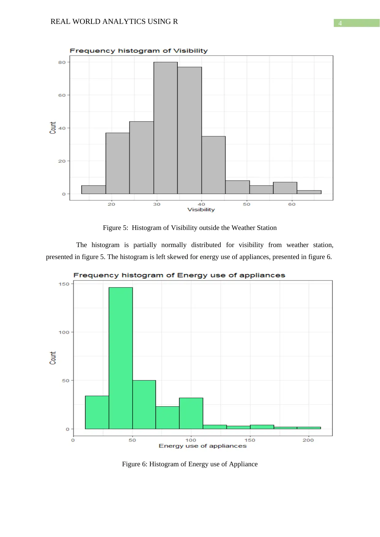
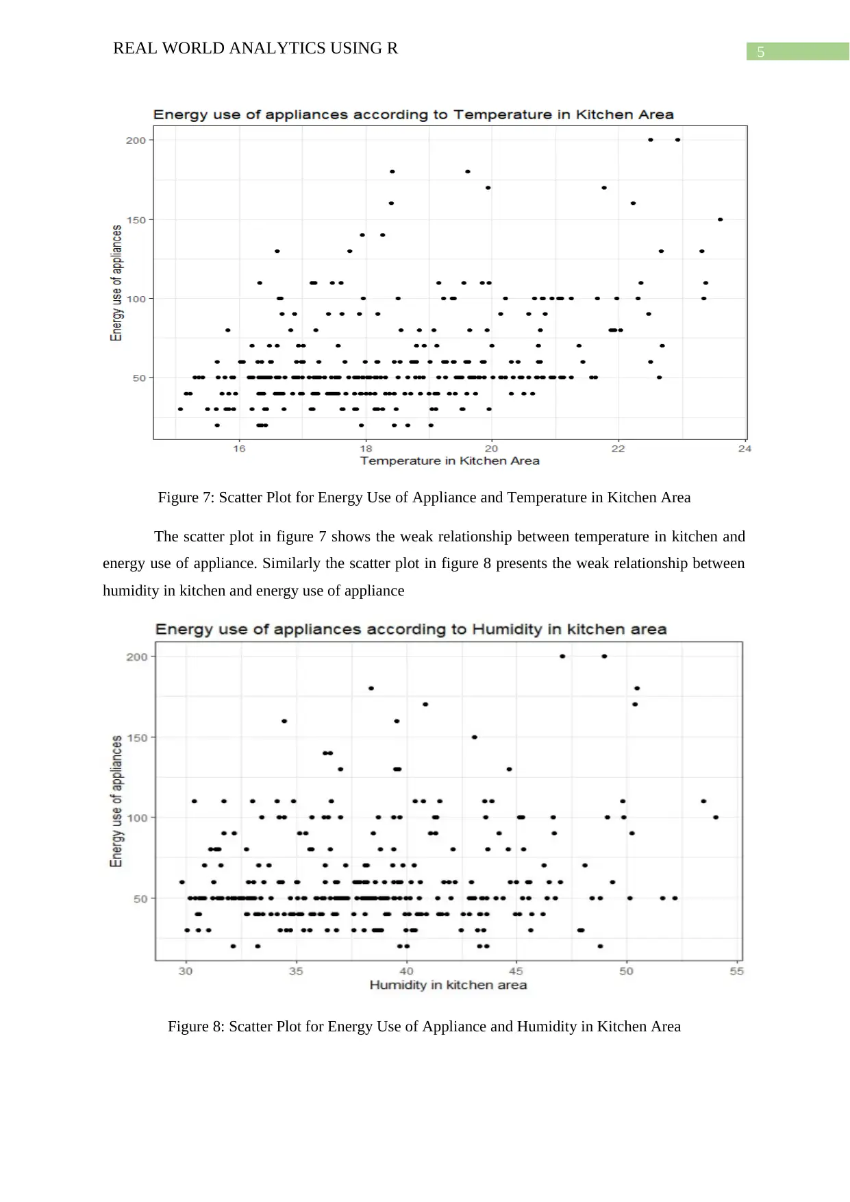
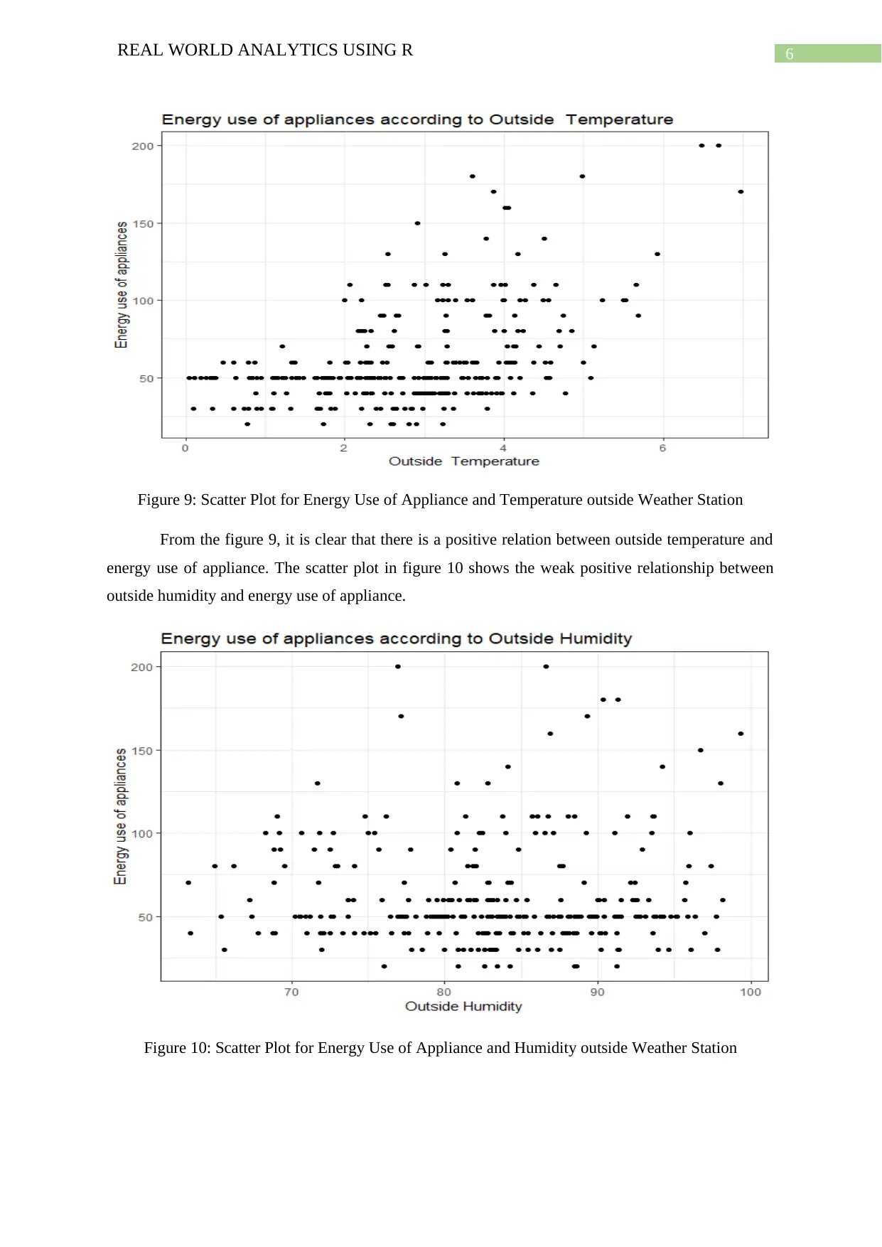
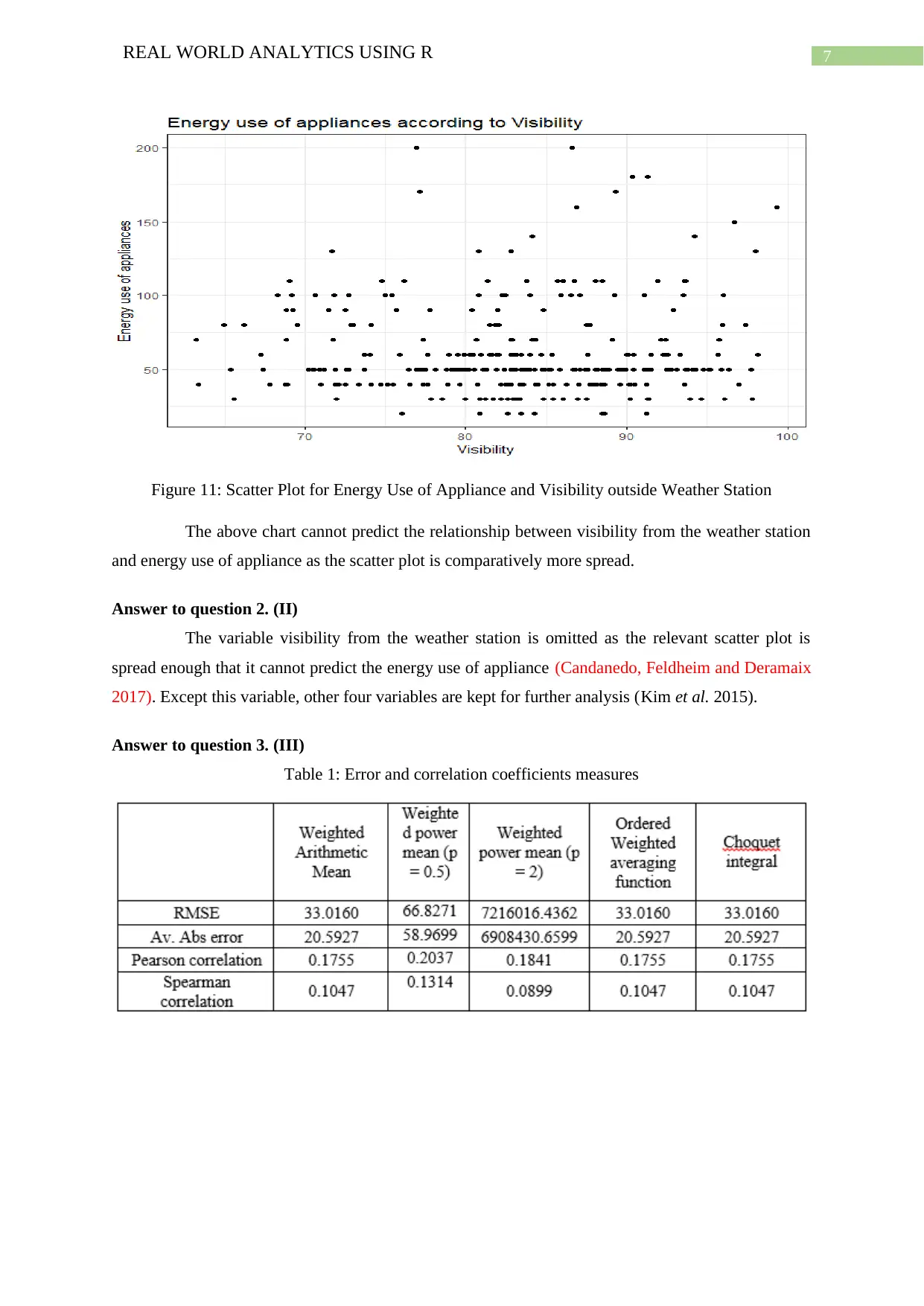
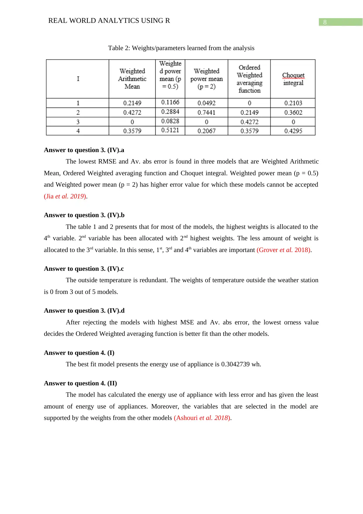
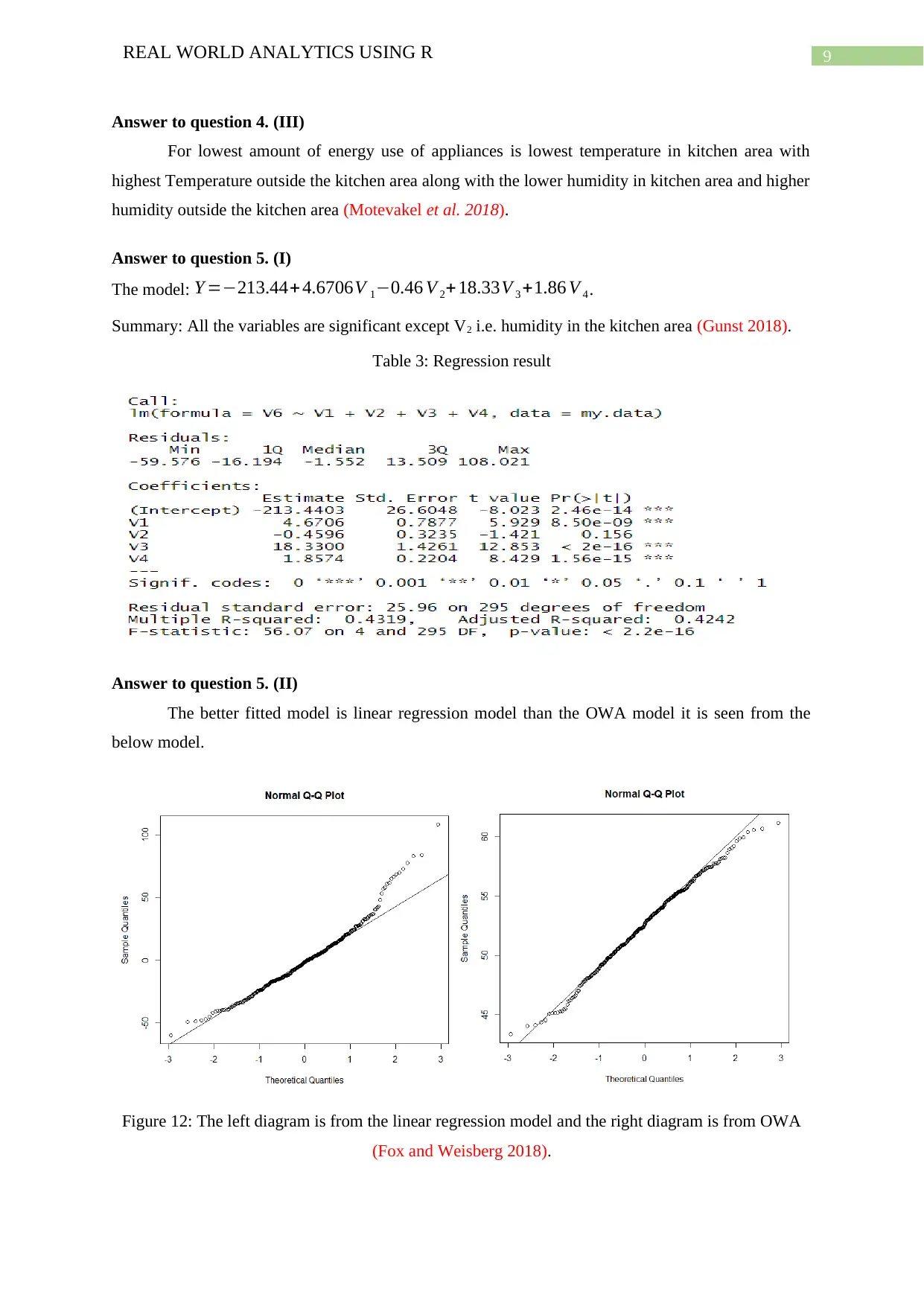
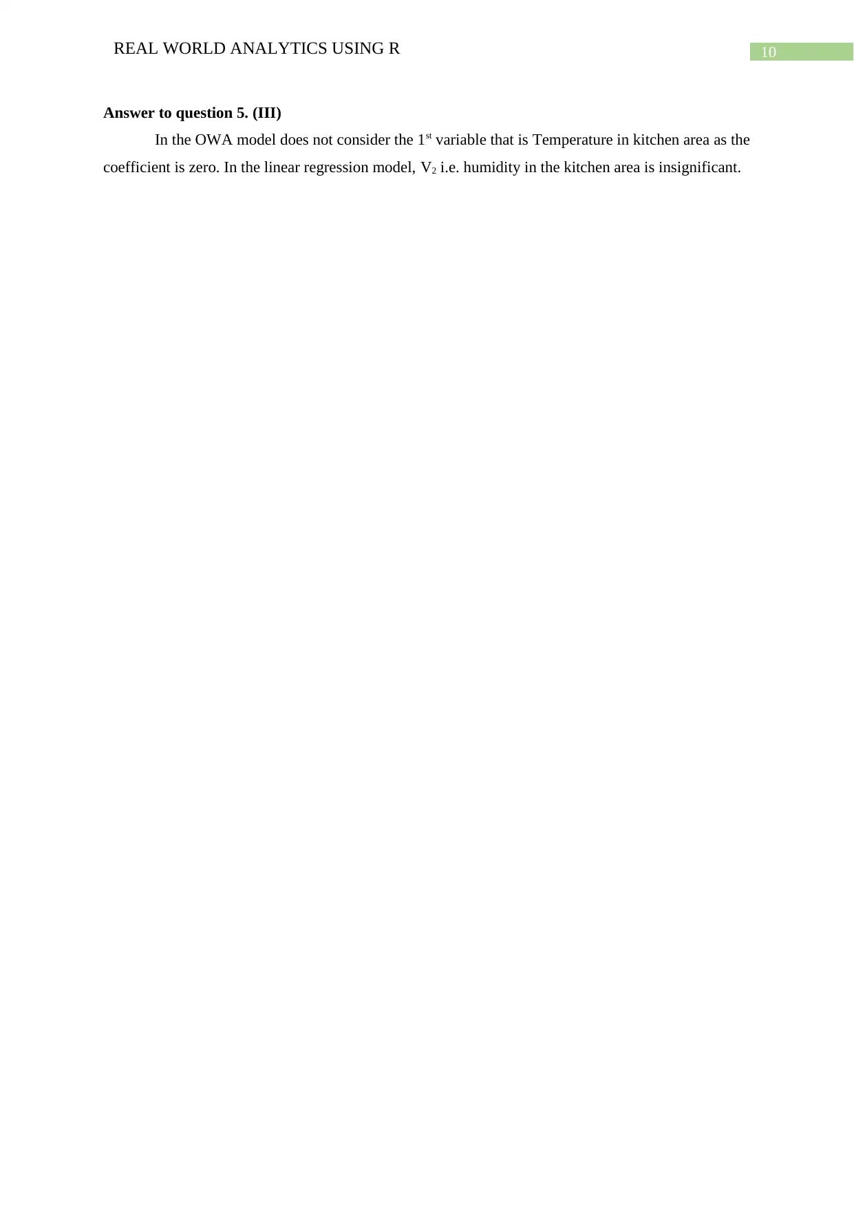
This report presents a comprehensive analysis of a real-world dataset using R, focusing on predicting energy use of appliances. The assignment explores data distributions, transformations, and the application of aggregation functions. It includes the creation of histograms and scatter plots to visualize relationships between variables such as temperature, humidity, and visibility with energy consumption. The report evaluates various models, including Weighted Arithmetic Mean, Ordered Weighted Averaging, and linear regression, based on error and correlation coefficients. It identifies significant variables, determines the best-fit model, and provides insights into the factors influencing energy use. The analysis also compares the performance of OWA and linear regression models, offering a detailed understanding of the dataset and the predictive capabilities of different analytical approaches. The assignment also includes the regression model, and provides insights into the relationships between the variables.

Running head: REAL WORLD ANALYTICS USING R
Real World Analytics Using R
Name of the Student:
Name of the University:
Author Note:

1REAL WORLD ANALYTICS USING R
Table of Contents
Answer to question 1. (IV)....................................................................................................................2
Answer to question 2. (II)......................................................................................................................7
Answer to question 3. (III).....................................................................................................................7
Answer to question 3. (IV).a..................................................................................................................8
Answer to question 3. (IV).b.................................................................................................................8
Answer to question 3. (IV).c..................................................................................................................8
Answer to question 3. (IV).d.................................................................................................................8
Answer to question 4. (I).......................................................................................................................8
Answer to question 4. (II)......................................................................................................................8
Answer to question 4. (III).....................................................................................................................8
Answer to question 5. (I).......................................................................................................................9
Answer to question 5. (II)......................................................................................................................9
Answer to question 5. (III).....................................................................................................................9
Reference and Bibliography................................................................................................................10

2REAL WORLD ANALYTICS USING R
Answer to question 1. (IV)
Figure 1: Histogram of Temperature in Kitchen Area (TKA)
The histogram is left skewed for temperature in kitchen area presented in figure 1. The
histogram is left skewed for humidity in kitchen area, presented in figure 2.
Figure 2: Histogram of Humidity in Kitchen Area (HKA)

3REAL WORLD ANALYTICS USING R
Figure 3: Histogram of Temperature outside Weather Station (TO)
The histogram is left skewed for temperature outside the weather station, presented in
figure 3. The histogram is right skewed for humidity outside the weather station, presented in figure 4.
Figure 4: Histogram of Humidity outside Weather Station (HO)

4REAL WORLD ANALYTICS USING R
Figure 5: Histogram of Visibility outside the Weather Station
The histogram is partially normally distributed for visibility from weather station,
presented in figure 5. The histogram is left skewed for energy use of appliances, presented in figure 6.
Figure 6: Histogram of Energy use of Appliance

5REAL WORLD ANALYTICS USING R
Figure 7: Scatter Plot for Energy Use of Appliance and Temperature in Kitchen Area
The scatter plot in figure 7 shows the weak relationship between temperature in kitchen and
energy use of appliance. Similarly the scatter plot in figure 8 presents the weak relationship between
humidity in kitchen and energy use of appliance
Figure 8: Scatter Plot for Energy Use of Appliance and Humidity in Kitchen Area

6REAL WORLD ANALYTICS USING R
Figure 9: Scatter Plot for Energy Use of Appliance and Temperature outside Weather Station
From the figure 9, it is clear that there is a positive relation between outside temperature and
energy use of appliance. The scatter plot in figure 10 shows the weak positive relationship between
outside humidity and energy use of appliance.
Figure 10: Scatter Plot for Energy Use of Appliance and Humidity outside Weather Station

7REAL WORLD ANALYTICS USING R
Figure 11: Scatter Plot for Energy Use of Appliance and Visibility outside Weather Station
The above chart cannot predict the relationship between visibility from the weather station
and energy use of appliance as the scatter plot is comparatively more spread.
Answer to question 2. (II)
The variable visibility from the weather station is omitted as the relevant scatter plot is
spread enough that it cannot predict the energy use of appliance (Candanedo, Feldheim and Deramaix
2017). Except this variable, other four variables are kept for further analysis (Kim et al. 2015).
Answer to question 3. (III)
Table 1: Error and correlation coefficients measures

8REAL WORLD ANALYTICS USING R
Table 2: Weights/parameters learned from the analysis
Answer to question 3. (IV).a
The lowest RMSE and Av. abs error is found in three models that are Weighted Arithmetic
Mean, Ordered Weighted averaging function and Choquet integral. Weighted power mean (p = 0.5)
and Weighted power mean (p = 2) has higher error value for which these models cannot be accepted
(Jia et al. 2019).
Answer to question 3. (IV).b
The table 1 and 2 presents that for most of the models, the highest weights is allocated to the
4th variable. 2nd variable has been allocated with 2nd highest weights. The less amount of weight is
allocated to the 3rd variable. In this sense, 1st, 3rd and 4th variables are important (Grover et al. 2018).
Answer to question 3. (IV).c
The outside temperature is redundant. The weights of temperature outside the weather station
is 0 from 3 out of 5 models.
Answer to question 3. (IV).d
After rejecting the models with highest MSE and Av. abs error, the lowest orness value
decides the Ordered Weighted averaging function is better fit than the other models.
Answer to question 4. (I)
The best fit model presents the energy use of appliance is 0.3042739 wh.
Answer to question 4. (II)
The model has calculated the energy use of appliance with less error and has given the least
amount of energy use of appliances. Moreover, the variables that are selected in the model are
supported by the weights from the other models (Ashouri et al. 2018).

9REAL WORLD ANALYTICS USING R
Answer to question 4. (III)
For lowest amount of energy use of appliances is lowest temperature in kitchen area with
highest Temperature outside the kitchen area along with the lower humidity in kitchen area and higher
humidity outside the kitchen area (Motevakel et al. 2018).
Answer to question 5. (I)
The model: Y =−213.44+ 4.6706V 1−0.46 V 2+ 18.33V 3 +1.86 V 4.
Summary: All the variables are significant except V2 i.e. humidity in the kitchen area (Gunst 2018).
Table 3: Regression result
Answer to question 5. (II)
The better fitted model is linear regression model than the OWA model it is seen from the
below model.
Figure 12: The left diagram is from the linear regression model and the right diagram is from OWA
(Fox and Weisberg 2018).

10REAL WORLD ANALYTICS USING R
Answer to question 5. (III)
In the OWA model does not consider the 1st variable that is Temperature in kitchen area as the
coefficient is zero. In the linear regression model, V2 i.e. humidity in the kitchen area is insignificant.

11REAL WORLD ANALYTICS USING R
Reference and Bibliography
Ashouri, M., Haghighat, F., Fung, B.C., Lazrak, A. and Yoshino, H., 2018. Development of building
energy saving advisory: A data mining approach. Energy and Buildings, 172, pp.139-151.
Fox, J. and Weisberg, S., 2018. An R companion to applied regression. Sage Publications.
Grover, V., Chiang, R.H., Liang, T.P. and Zhang, D., 2018. Creating strategic business value from big
data analytics: A research framework. Journal of Management Information Systems, 35(2), pp.388-
423.
Gunst, R.F., 2018. Regression analysis and its application: a data-oriented approach. Routledge.
Jia, K., Guo, G., Xiao, J., Zhou, H., Wang, Z. and He, G., 2019. Data compression approach for the
home energy management system. Applied Energy, 247, pp.643-656.
Kim, H., Choo, J., Park, H. and Endert, A., 2015. Interaxis: Steering scatterplot axes via observation-
level interaction. IEEE transactions on visualization and computer graphics, 22(1), pp.131-140.
Candanedo, L.M., Feldheim, V. and Deramaix, D., 2017. Data driven prediction models of energy use
of appliances in a low-energy house. Energy and buildings, 140, pp.81-97.
Motevakel, P., Ghanbari, B., Abedi, M. and Hosseinian, S.H., 2018, November. Demand-Side Energy
Management in an Administrative Building by Considering Generation Optimization. In 2018 Smart
Grid Conference (SGC) (pp. 1-6). IEEE.