Deakin University SIT718 Real World Analytics: Problem Solving Project

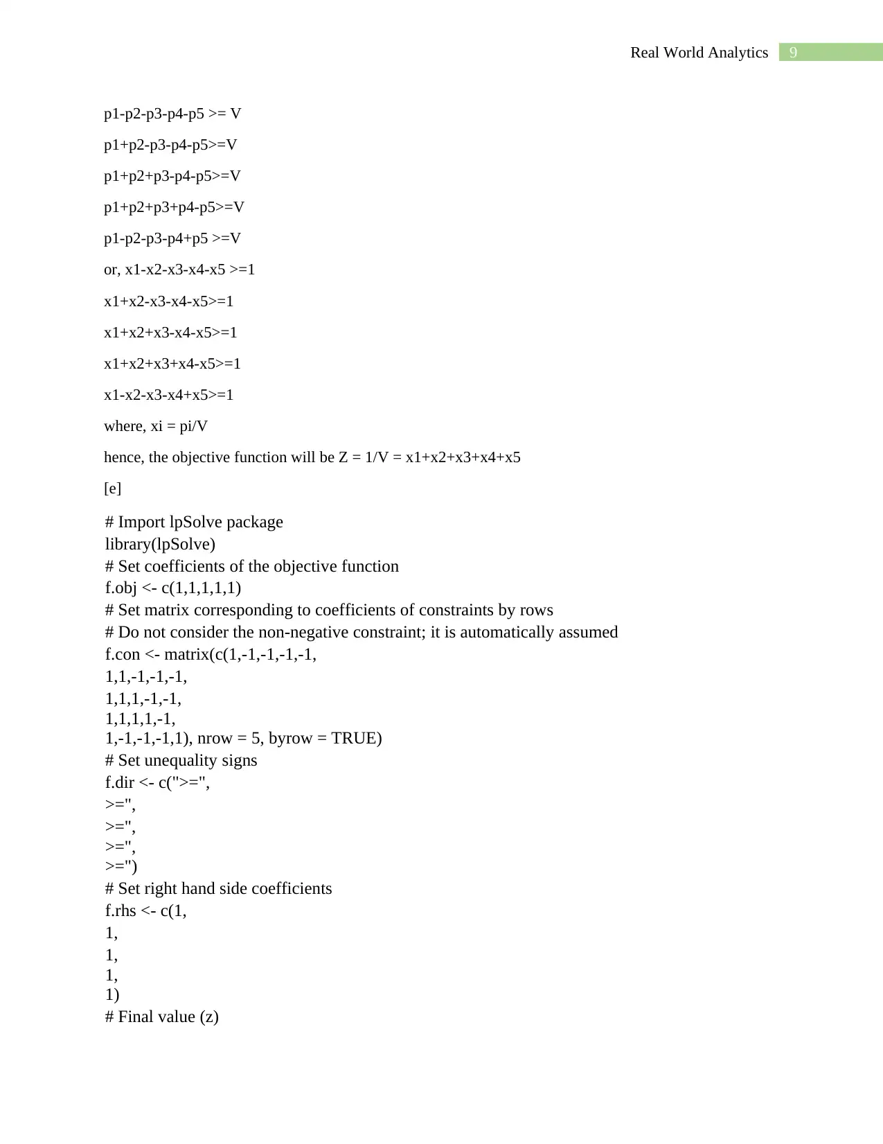
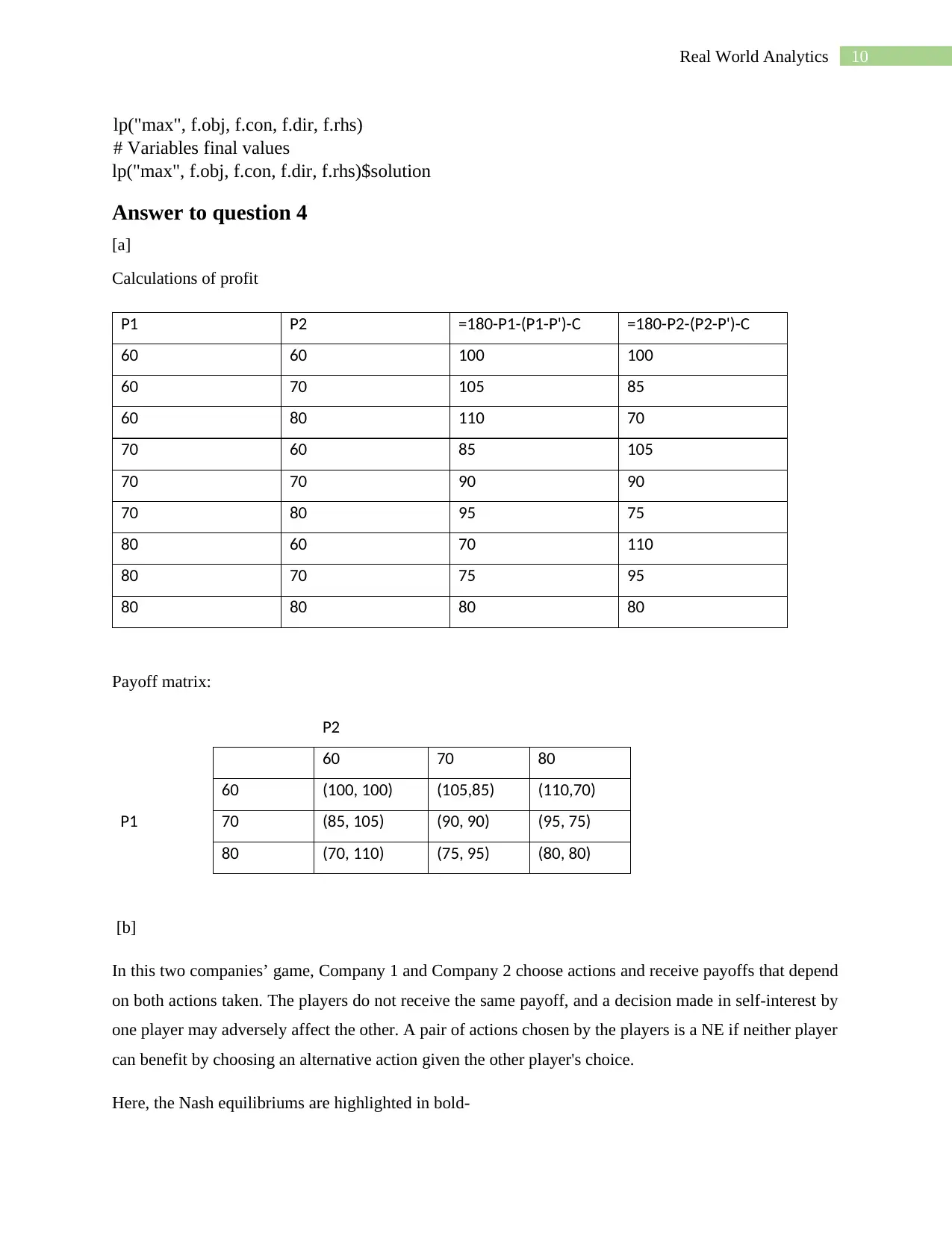
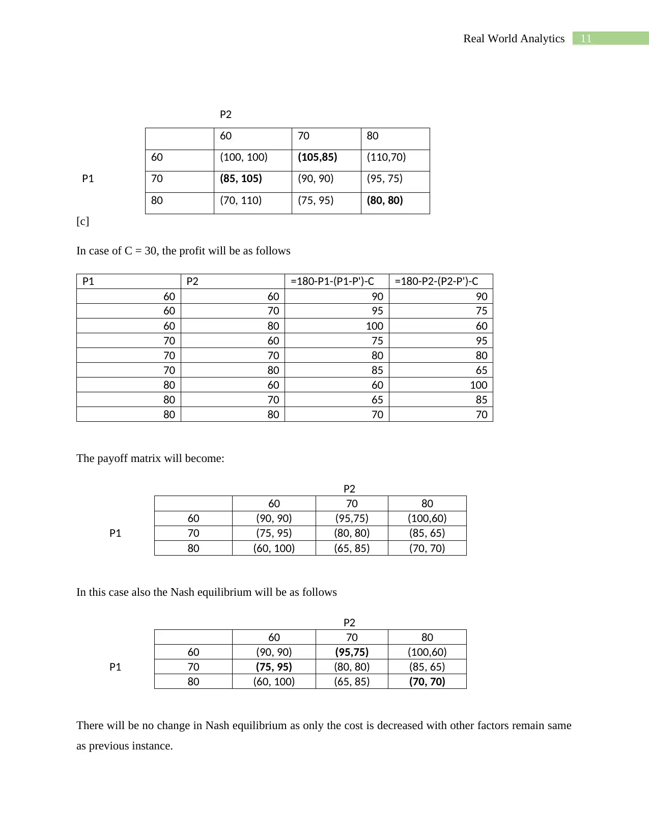
This assignment, part of the SIT718 Real World Analytics course at Deakin University, focuses on applying linear programming and game theory to solve real-world problems. The project requires students to build and solve linear programming models, including those with two variables using graphical methods and those with more variables using software like R. The assignment also explores game theory, specifically two-player zero-sum games, by constructing payoff matrices and identifying Nash equilibriums. Students are tasked with analyzing different bidding scenarios and determining optimal strategies for companies. The solution provided covers various aspects of linear programming, including constraint optimization, and provides code for solving these problems using the R programming language. The assignment assesses the student's ability to apply these techniques to make optimal decisions and develop software code for computational problem solving. The solution provided covers various aspects of linear programming, including constraint optimization, and provides code for solving these problems using the R programming language. The assignment assesses the student's ability to apply these techniques to make optimal decisions and develop software code for computational problem solving.

Running head: Real World Analytics
Real world Analytics
Student Name:
Student ID:
University Name:
Paper Code:

2Real World Analytics
Table of Contents
Answer to question 1.................................................................................................................................3
Answer to question 2.................................................................................................................................4
Answer to question 3.................................................................................................................................7
Answer to question 4...............................................................................................................................10
References................................................................................................................................................13

3Real World Analytics
Answer to question 1
1.a)
Linear programming is considered to be a programming model which is an algebraic description
which is the main aim that is to be maximize or minimize the constraint that need to be satisfied by the
variable. Linear programming techniques helps in improving the quality of decisions.
Linear programing has given a way to unify results which are the mechanism design from
disparate areas. Linear programming is another crucial and important part of mathematics that deals with
the study of optimization problem with the required number of constraints and objective. To find a point
which is in the polyhedron where the function has the smallest or it can be said that the largest value if
exist.
1.b)
Let x be the invested amount from factory A.
Let y be the invested amount from factory B.
To optimize Z=5x+8y
The recipes for the production of the new cheese require
30x+80y<=60
60x+40y>=45
40x+70y>=50
These are the restriction
Hence,
To optimize Z = 5x+8y
Subject to the constraints
30x+80y<=60
60x+40y>=45
40x+70y>=50
1.c)
To solve this problem let us consider the in equations as equations as follow:
30x+80y = 60 …(1)
60x+40y = 45 …(2)
40x+70y = 50 ….(3)
Now, putting these equations in graph, we have,

4Real World Analytics
Figure 1
The graph have been solved from online graph maker available
From the above graph, we can say the feasible region is ABCDA.
Now, we have the coordinates of A, B, C and D are (23/52 , 6/13), (1/3 , 5/8), (0 , ¾), (0 , 5/7)
respectively.
Now, at A, Z = 5*(23/52)+8*(6/13) = 5.90
At B, Z = 5*(1/3)+8*(5/8) = 6.67
At C, Z = 5*(0)+8*(3/4) =6
And at D, Z = 5*0 + 8*(5/7) = 5.71
Hence, D will be the minimum point.
It means, the optimum solution is (0 , 5/7)
Answer to question 2
2.a)
xc1/(xc1+xw1+xs1) Cotton in Spring =>y1>=0.5

5Real World Analytics
xc2/(xc2+xw2+xs2) Cotton in Autumn =>y2>=0.6
xc3/(xc3+xw3+xs3) Cotton in Winter =>y3>=0.4
xw1/(xc1+xw1+xs1) Wool in Spring =>y4>=0.4
xw2/(xc2+xw2+xs2) Wool in Autumn =>y5>=0.4
xw3/(xc3+xw3+xs3) Wool in Winter =>y6>=0.5
xs1/(xc1+xw1+xs1) Silk in Spring =>y7
xs2/(xc2+xw2+xs2) Silk in Spring =>y8
xs3/(xc2+xw2+xs2) Silk in Spring =>y9
For spring => (y1+y4+y7)<=4200
For autumn => (y2+y5+y8)<=3200
For winter => (y3+y6+y9)<=3500
Thus,
=55(y1+y4+y7)-30(y1+y2+y3)+51(y2+y5+y8)-45(y4+y5+y6)+55(y3+y6+y9)-50(y7+y8+y9)
=25y1+21y2+25y3+10y4+6y5+10y6+5y7+y8+5y9
Thus the linear equation looks like below-
Max Z= 25y1+21y2+25y3+10y4+6y5+10y6+5y7+y8+5y9
Subject to:
1y1+0y2+0y3+0y4+0y5+0y6+0y7+0y8+0y9>=.5
0y1+1y2+0y3+0y4+0y5+0y6+0y7+0y8+0y9>=.6
0y1+0y2+1y3+0y4+0y5+0y6+0y7+0y8+0y9>=.4
0y1+0y2+0y3+1y4+0y5+0y6+0y7+0y8+0y9>=.4
0y1+0y2+0y3+0y4+1y5+0y6+0y7+0y8+0y9>=.4
0y1+0y2+0y3+0y4+0y5+1y6+0y7+0y8+0y9>=.5
1y1+0y2+0y3+1y4+0y5+0y6+1y7+0y8+0y9<=4200
0y1+1y2+0y3+0y4+1y5+0y6+0y7+1y8+0y9<=3200
0y1+0y2+1y3+0y4+0y5+1y6+0y7+0y8+1y9<=3500
For maximizing the profit these formulas need to be solved using linear programming.
2.b)
# Import lpSolve package
library(lpSolve)

6Real World Analytics
# Set coefficients of the objective function
f.obj <- c(25 , 21 , 25 , 10 , 6 , 10 ,
5 , 1 , 5
)
# Set matrix corresponding to coefficients of constraints by rows
# Do not consider the non-negative constraint; it is automatically assumed
f.con <- matrix(c(1 , 0 , 0 , 0 , 0 , 0
, 0 , 0 , 0 ,
0 , 1 , 0 , 0 , 0 , 0 , 0
, 0 , 0 ,
0 , 0 , 1 , 0 , 0 , 0 , 0
, 0 , 0 ,
0 , 0 , 0 , 1 , 0 , 0 , 0
, 0 , 0 ,
0 , 0 , 0 , 0 , 1 , 0 , 0
, 0 , 0 ,
0 , 0 , 0 , 0 , 0 , 1 , 0
, 0 , 0 ,
1 , 0 , 0 , 1 , 0 , 0 , 1
, 0 , 0 ,
0 , 1 , 0 , 0 , 1 , 0 , 0
, 1 , 0 ,
0 , 0 , 1 , 0 , 0 , 1 , 0
, 0 , 1
), nrow = 9, byrow = TRUE)
# Set unequality signs
f.dir <- c(">=",
">=",
">=",
">=",
">=",
">=",
"<=",
"<=",

7Real World Analytics
"<=")
# Set right hand side coefficients
f.rhs <- c(0.5,
0.6,
0.4,
0.4,
0.4,
0.5,
4200,
3200,
3500)
# Final value (z)
lp("max", f.obj, f.con, f.dir, f.rhs)
# Variables final values
lp("max", f.obj, f.con, f.dir, f.rhs)$solution
Answer to question 3
[a]
The can be considered as two-players-zero-sum game as the terms (or coordinates) in each payoff
vector must add up to the same value for each payoff vector which is what we can see from the payoff
matrix. It is called so because one player wins whatever the other player loses.
[b]
Playoff matrix
Let C1 denotes company 1 wins and C2 denotes company 2 wins. Hence, considering all bidding options,
following is the play off matrix.
C2
Play off matrix 10 20 30 40 50
C1
10 (10,10) (10,20) (10,30) (10,40) (10,50)
20 (20,10) (20,20) (20,30) (20,40) (20,50)
30 (30,10) (30,20) (30,30) (30,40) (30,50)
40 (40,10) (40,20) (40,30) (40,40) (40,50)
50 (50,10) (50,20) (50,30) (50,40) (50,50)

8Real World Analytics
C2
10 20 30 40 50
C1
10 1 -1 -1 -1 -1
20 1 1 -1 -1 -1
30 1 1 1 -1 -1
40 1 1 1 1 -1
50 1 -1 -1 -1 1
[c]
If some entry aij of the matrix A has the property that
(1) aij is the minimum of the ith row, and
(2) aij is the maximum of the jth column,
Then we say aij is a saddle point.
C2
10 20 30 40 50 Row Min
C1
10 1 -1 -1 -1 -1 -1
20 1 1 -1 -1 -1 -1
30 1 1 1 -1 -1 -1
40 1 1 1 1 -1 -1
50 1 -1 -1 -1 1 -1
Column Max 1 1 1 1 1
Here, column MaxiMin ≠ Row MiniMax
∴ This game has no saddle point.
[d]
Let V = value of the game
p1,p2,p3, p4, p5 = probabilities of selecting strategies C1a, C1b, C1c, C1d, C1e respectively.
q1,q2,q3, q4, q5 = probabilities of selecting strategies C2a, C2b, C2c, C2d, C2e respectively.

9Real World Analytics
p1-p2-p3-p4-p5 >= V
p1+p2-p3-p4-p5>=V
p1+p2+p3-p4-p5>=V
p1+p2+p3+p4-p5>=V
p1-p2-p3-p4+p5 >=V
or, x1-x2-x3-x4-x5 >=1
x1+x2-x3-x4-x5>=1
x1+x2+x3-x4-x5>=1
x1+x2+x3+x4-x5>=1
x1-x2-x3-x4+x5>=1
where, xi = pi/V
hence, the objective function will be Z = 1/V = x1+x2+x3+x4+x5
[e]
# Import lpSolve package
library(lpSolve)
# Set coefficients of the objective function
f.obj <- c(1,1,1,1,1)
# Set matrix corresponding to coefficients of constraints by rows
# Do not consider the non-negative constraint; it is automatically assumed
f.con <- matrix(c(1,-1,-1,-1,-1,
1,1,-1,-1,-1,
1,1,1,-1,-1,
1,1,1,1,-1,
1,-1,-1,-1,1), nrow = 5, byrow = TRUE)
# Set unequality signs
f.dir <- c(">=",
>=",
>=",
>=",
>=")
# Set right hand side coefficients
f.rhs <- c(1,
1,
1,
1,
1)
# Final value (z)

10Real World Analytics
lp("max", f.obj, f.con, f.dir, f.rhs)
# Variables final values
lp("max", f.obj, f.con, f.dir, f.rhs)$solution
Answer to question 4
[a]
Calculations of profit
P1 P2 =180-P1-(P1-P')-C =180-P2-(P2-P')-C
60 60 100 100
60 70 105 85
60 80 110 70
70 60 85 105
70 70 90 90
70 80 95 75
80 60 70 110
80 70 75 95
80 80 80 80
Payoff matrix:
P2
60 70 80
P1
60 (100, 100) (105,85) (110,70)
70 (85, 105) (90, 90) (95, 75)
80 (70, 110) (75, 95) (80, 80)
[b]
In this two companies’ game, Company 1 and Company 2 choose actions and receive payoffs that depend
on both actions taken. The players do not receive the same payoff, and a decision made in self-interest by
one player may adversely affect the other. A pair of actions chosen by the players is a NE if neither player
can benefit by choosing an alternative action given the other player's choice.
Here, the Nash equilibriums are highlighted in bold-

11Real World Analytics
P2
60 70 80
P1
60 (100, 100) (105,85) (110,70)
70 (85, 105) (90, 90) (95, 75)
80 (70, 110) (75, 95) (80, 80)
[c]
In case of C = 30, the profit will be as follows
P1 P2 =180-P1-(P1-P')-C =180-P2-(P2-P')-C
60 60 90 90
60 70 95 75
60 80 100 60
70 60 75 95
70 70 80 80
70 80 85 65
80 60 60 100
80 70 65 85
80 80 70 70
The payoff matrix will become:
P2
60 70 80
P1
60 (90, 90) (95,75) (100,60)
70 (75, 95) (80, 80) (85, 65)
80 (60, 100) (65, 85) (70, 70)
In this case also the Nash equilibrium will be as follows
P2
60 70 80
P1
60 (90, 90) (95,75) (100,60)
70 (75, 95) (80, 80) (85, 65)
80 (60, 100) (65, 85) (70, 70)
There will be no change in Nash equilibrium as only the cost is decreased with other factors remain same
as previous instance.

12Real World Analytics
References
Braun, W.J. and Murdoch, D.J., 2016. A first course in statistical programming with R. Cambridge
University Press.
Fearnley, J. and Savani, R., 2015, June. The complexity of the simplex method. In Proceedings of the
forty-seventh annual ACM symposium on Theory of computing (pp. 201-208).
Ficken, F.A., 2015. The simplex method of linear programming. Courier Dover Publications.
Fletcher, R., 2013. Practical methods of optimization. John Wiley & Sons.
Sallan, J.M., Lordan, O. and Fernandez, V., 2015. Modeling and solving linear programming with R.
OmniaScience.
Vanderbei, R.J., 2015. Linear programming. Heidelberg: Springer.