SIT718 Real World Analytics Assignment 4: Linear Programming
VerifiedAdded on 2022/11/01
|17
|2909
|404
Homework Assignment
AI Summary
This document presents a comprehensive solution to Assignment 4 of the SIT718 Real World Analytics course, focusing on the application of linear programming and game theory. The assignment addresses several real-world scenarios, including cost minimization in a beverage production context, profit maximization in a manufacturing setting, and the analysis of a two-player zero-sum game. The solution utilizes mathematical modeling, graphical methods, and software like R-studio to solve the problems, including formulating linear programs, defining constraints, and determining optimal strategies. The solution also includes an analysis of a game theory payoff matrix and the identification of Nash equilibrium. The assignment demonstrates the practical application of these analytical tools in decision-making processes across different business scenarios.
Assignment: Analytic 1
ASSIGNMENT 4
by[Name]
Course
Professor’s Name
Institution
Location of Institution
Date
ASSIGNMENT 4
by[Name]
Course
Professor’s Name
Institution
Location of Institution
Date
Paraphrase This Document
Need a fresh take? Get an instant paraphrase of this document with our AI Paraphraser
Assignment: Analytic 2
Assignment 4
Question 1
(a) The basic requirement for a problem to be solved using linear programming method is
that the problem must be of maximization or minimization of linear objective function
subject to a set of linear constraints (Akpinar and Baykasoglu 2014; Higle and Sen
2013; Recht, Re and Bittorf 2012). The factory needs to minimize cost given the
linear combination of cost of each product needed to make the beverage. Therefore,
the fundamental requirement for a problem to be modelled by linear program is met
(minimization). In addition to the basic requirement there are other four more
assumptions that should be satisfied for the problem to be modelled using LP.
1) Proportionality – each products cost has a direct impact of the final cost of the
beverage thus the assumption is satisfied (Akpinar and Baykasoglu 2014). 2)
additivity - the decision on how many units of product A to use is independent of that
for product B. Thus, the contribution to the objective function for any product is
independent of the other. 3) divisibility- the variables being used in the decision
criteria are continuous for instance the customer requires a minimum of 4.5 liters of
orange. An indication that fractional units can be used. 4) certainty – the factory
cannot produce negative volumes of beverage since the customer requires a minimum
of 80 liters per week and it cannot use less than zero units of the products A and B.
(b) Suppose the factory use x = liters of product A and y liters of product B in making (x
+ y) liters of the beverage. Then, it implies that the total cost of producing (x + y)
liters of beverage is
C = 5x + 7y. (i)
Assignment: Analytic 3
Also, we know that liters of orange must not less than 4.5 liters in 100 liters of
beverage giving us equation (ii).
0.06 x +0.04 y ≥ 4.5 which simplifies to 3 x+ 2 y ≥ 225 (ii)
Next, mango used should not be less than 5 liters per 100liters of beverage
0.04 x +0.06 y ≥5 which simplifies to 2 x+3 y ≥ 250 (iii)
Similarly, lime used at most 6 liters per 100liters of beverage
0.03 x+0.08 y ≤ 6 which simplifies to 3x +8 y ≤ 600 (iv)
But the customer also has some demands as follows
x + y ≥ 80 (v)
Certainty constraints
x ≥ 0 and y≥ 0 form equation (vi) and (vii).
Therefore, the LP is to minimize equation (i) subject to constraints presented in
equation (ii) to (vii). That is
Min C = 5x + 7y.
Subject to:
3 x+ 2 y ≥ 225
2 x+3 y ≥ 250
3 x +8 y ≤ 600
x + y ≥ 80
x ≥ 0 and y≥ 0
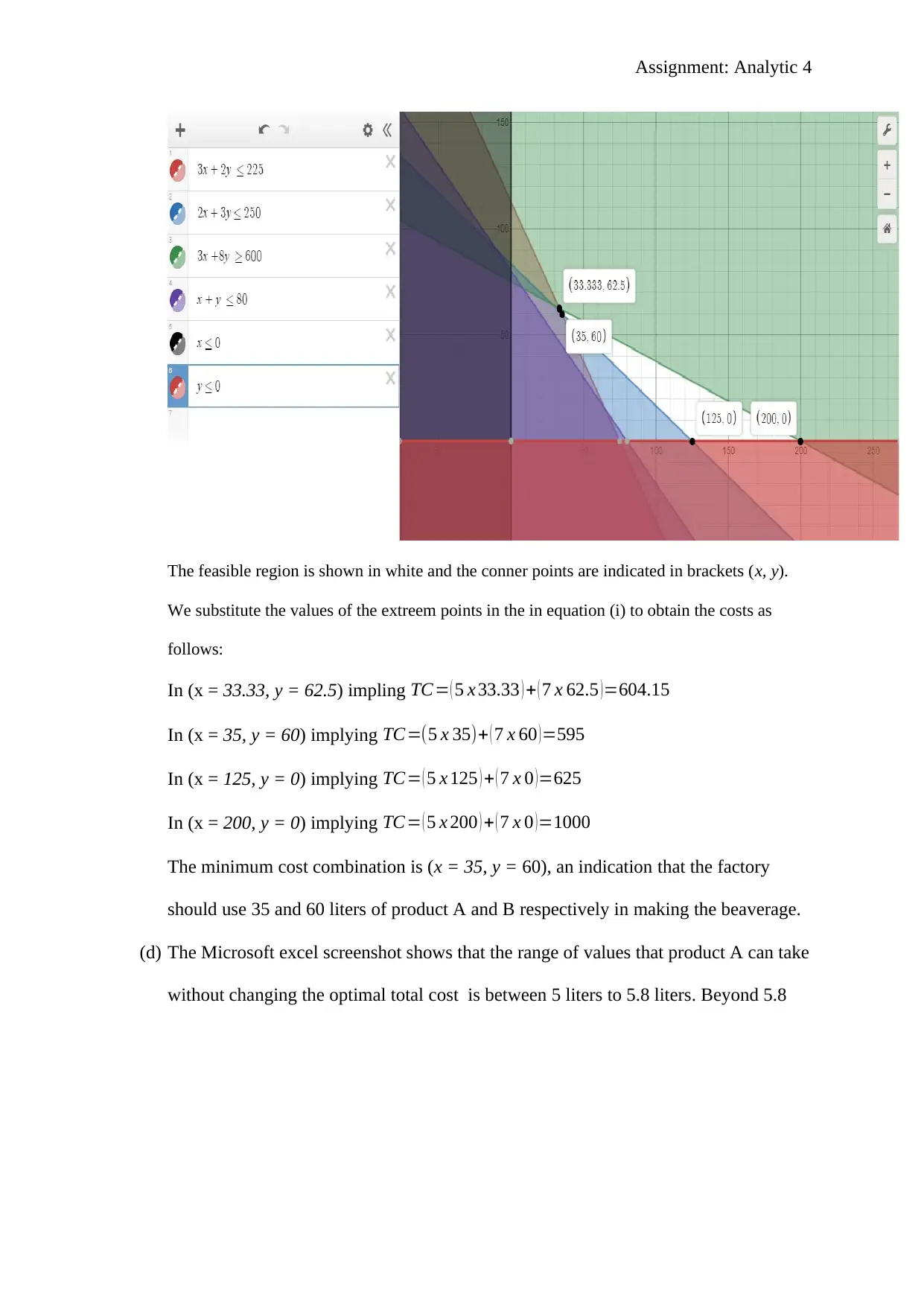
(c) In plotting the inequalities, we input the signs in the reverse order (if ≥ we input ≤) in
the desmos.com function plotting platform (Desmos.com). The plotted graph is
shown below
Also, we know that liters of orange must not less than 4.5 liters in 100 liters of
beverage giving us equation (ii).
0.06 x +0.04 y ≥ 4.5 which simplifies to 3 x+ 2 y ≥ 225 (ii)
Next, mango used should not be less than 5 liters per 100liters of beverage
0.04 x +0.06 y ≥5 which simplifies to 2 x+3 y ≥ 250 (iii)
Similarly, lime used at most 6 liters per 100liters of beverage
0.03 x+0.08 y ≤ 6 which simplifies to 3x +8 y ≤ 600 (iv)
But the customer also has some demands as follows
x + y ≥ 80 (v)
Certainty constraints
x ≥ 0 and y≥ 0 form equation (vi) and (vii).
Therefore, the LP is to minimize equation (i) subject to constraints presented in
equation (ii) to (vii). That is
Min C = 5x + 7y.
Subject to:
3 x+ 2 y ≥ 225
2 x+3 y ≥ 250
3 x +8 y ≤ 600
x + y ≥ 80
x ≥ 0 and y≥ 0
(c) In plotting the inequalities, we input the signs in the reverse order (if ≥ we input ≤) in
the desmos.com function plotting platform (Desmos.com). The plotted graph is
shown below
⊘ This is a preview!⊘
Do you want full access?
Subscribe today to unlock all pages.
Trusted by 1+ million students worldwide
Assignment: Analytic 4
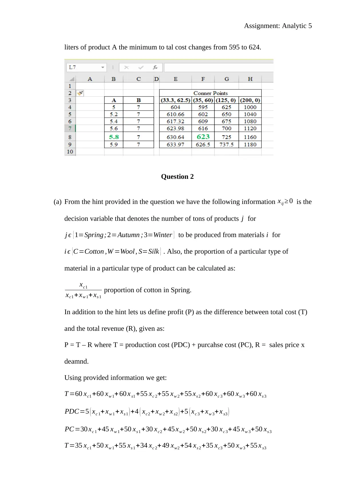
The feasible region is shown in white and the conner points are indicated in brackets (x, y).
We substitute the values of the extreem points in the in equation (i) to obtain the costs as
follows:
In (x = 33.33, y = 62.5) impling TC= ( 5 x 33.33 ) + ( 7 x 62.5 )=604.15
In (x = 35, y = 60) implying TC=(5 x 35)+ ( 7 x 60 )=595
In (x = 125, y = 0) implying TC= ( 5 x 125 ) + ( 7 x 0 )=625
In (x = 200, y = 0) implying TC= ( 5 x 200 ) + ( 7 x 0 ) =1000
The minimum cost combination is (x = 35, y = 60), an indication that the factory
should use 35 and 60 liters of product A and B respectively in making the beaverage.
(d) The Microsoft excel screenshot shows that the range of values that product A can take
without changing the optimal total cost is between 5 liters to 5.8 liters. Beyond 5.8
Paraphrase This Document
Need a fresh take? Get an instant paraphrase of this document with our AI Paraphraser
Assignment: Analytic 5
liters of product A the minimum to tal cost changes from 595 to 624.
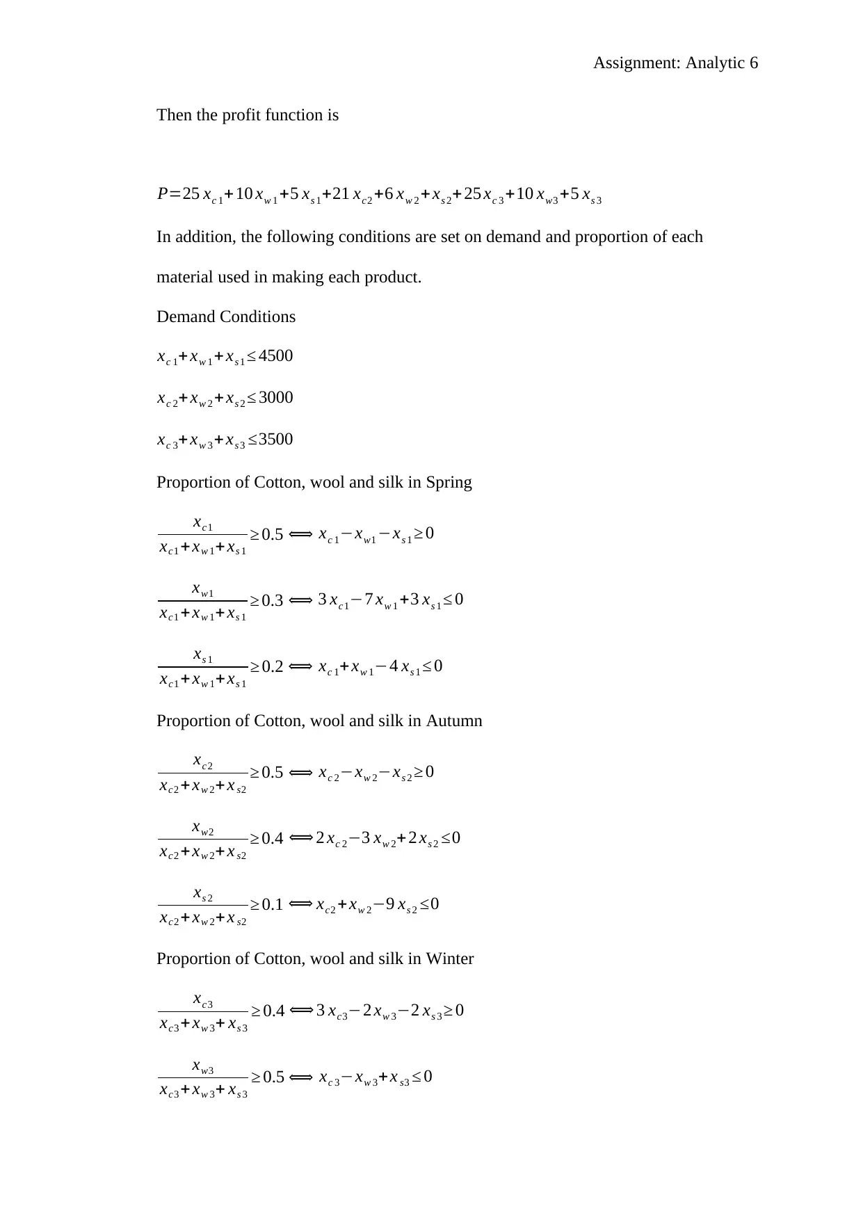
Question 2
(a) From the hint provided in the question we have the following information xij ≥ 0 is the
decision variable that denotes the number of tons of products j for
j ϵ { 1=Spring;2=Autumn ; 3=Winter } to be produced from materials i for
i ϵ {C=Cotton ,W =Wool , S=Silk } . Also, the proportion of a particular type of
material in a particular type of product can be calculated as:
xc1
xc1 +xw 1+ xs 1
proportion of cotton in Spring.
In addition to the hint lets us define profit (P) as the difference between total cost (T)
and the total revenue (R), given as:
P = T – R where T = production cost (PDC) + purcahse cost (PC), R = sales price x
deamnd.
Using provided information we get:
T =60 xc1 +60 xw 1+ 60 x s1 +55 xc 2+55 xw 2+55 xs 2 +60 xc 3+60 xw 3 +60 xs 3
PDC=5 ( xc 1+ xw 1 + xs 1 ) +4 ( xc2 + xw 2+ x s2 ) +5 ( xc 3 + xw 3+x s3 )
PC =30 xc 1 +45 xw 1+50 xs 1 +30 xc2 + 45 xw 2 +50 xs 2+30 xc 3+ 45 xw 3+50 xs 3
T =35 xc1 +50 xw 1+55 xs 1 +34 xc 2+ 49 xw2 +54 xs 2 +35 xc3 +50 xw 3+ 55 x s3
liters of product A the minimum to tal cost changes from 595 to 624.
Question 2
(a) From the hint provided in the question we have the following information xij ≥ 0 is the
decision variable that denotes the number of tons of products j for
j ϵ { 1=Spring;2=Autumn ; 3=Winter } to be produced from materials i for
i ϵ {C=Cotton ,W =Wool , S=Silk } . Also, the proportion of a particular type of
material in a particular type of product can be calculated as:
xc1
xc1 +xw 1+ xs 1
proportion of cotton in Spring.
In addition to the hint lets us define profit (P) as the difference between total cost (T)
and the total revenue (R), given as:
P = T – R where T = production cost (PDC) + purcahse cost (PC), R = sales price x
deamnd.
Using provided information we get:
T =60 xc1 +60 xw 1+ 60 x s1 +55 xc 2+55 xw 2+55 xs 2 +60 xc 3+60 xw 3 +60 xs 3
PDC=5 ( xc 1+ xw 1 + xs 1 ) +4 ( xc2 + xw 2+ x s2 ) +5 ( xc 3 + xw 3+x s3 )
PC =30 xc 1 +45 xw 1+50 xs 1 +30 xc2 + 45 xw 2 +50 xs 2+30 xc 3+ 45 xw 3+50 xs 3
T =35 xc1 +50 xw 1+55 xs 1 +34 xc 2+ 49 xw2 +54 xs 2 +35 xc3 +50 xw 3+ 55 x s3
Assignment: Analytic 6
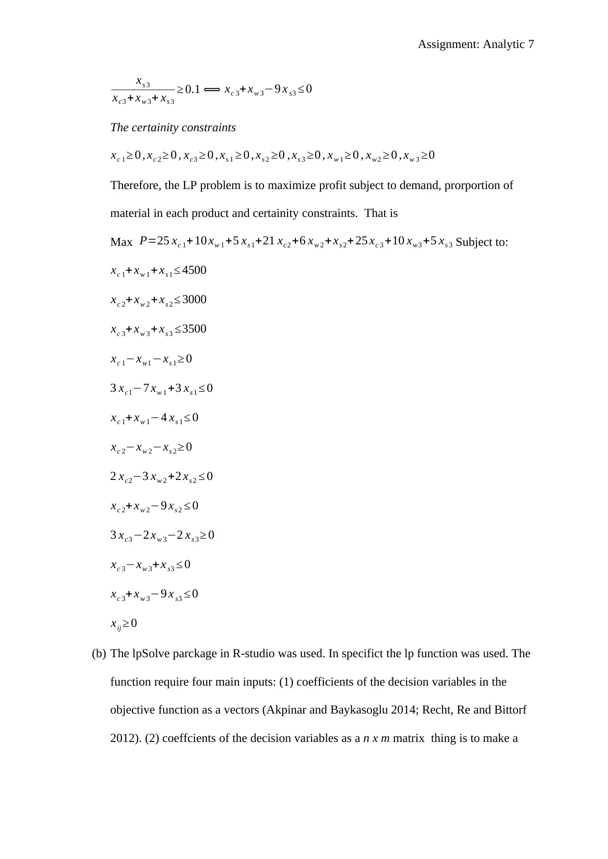
Then the profit function is
P=25 xc 1+ 10 xw 1 +5 xs 1+21 xc2 +6 xw 2 + xs 2+ 25 xc 3 +10 xw3 +5 xs 3
In addition, the following conditions are set on demand and proportion of each
material used in making each product.
Demand Conditions
xc 1+xw 1 + xs 1 ≤ 4500
xc 2+ xw 2 +xs 2 ≤ 3000
xc 3+xw 3 + xs 3 ≤3500
Proportion of Cotton, wool and silk in Spring
xc1
xc1 +xw 1+ xs 1
≥ 0.5 ⟺ xc 1−xw1 −xs 1 ≥ 0
xw1
xc1 + xw 1+ xs 1
≥ 0.3 ⟺ 3 xc1−7 xw 1 +3 xs 1 ≤ 0
xs 1
xc1 + xw 1+xs 1
≥ 0.2 ⟺ xc 1+ xw 1−4 xs 1 ≤ 0
Proportion of Cotton, wool and silk in Autumn
xc2
xc2 + xw 2+ x s2
≥ 0.5 ⟺ xc 2−xw 2−xs 2 ≥ 0
xw2
xc2 +xw 2+ x s2
≥ 0.4 ⟺ 2 xc 2−3 xw 2+ 2 xs 2 ≤0
xs 2
xc2 + xw 2+ x s2
≥ 0.1 ⟺ xc2 +xw 2−9 xs 2 ≤0
Proportion of Cotton, wool and silk in Winter
xc3
xc3 + xw 3+ xs 3
≥ 0.4 ⟺ 3 xc3−2 xw 3−2 xs 3 ≥ 0
xw3
xc3 + xw 3+ xs 3
≥ 0.5 ⟺ xc 3−xw 3+x s3 ≤ 0
⊘ This is a preview!⊘
Do you want full access?
Subscribe today to unlock all pages.
Trusted by 1+ million students worldwide
Assignment: Analytic 7
xs 3
xc3 +xw 3+ xs 3
≥ 0.1 ⟺ xc 3+xw 3−9 x s3 ≤ 0
The certainity constraints
xc 1 ≥ 0 , xc 2 ≥ 0 , xc3 ≥ 0 , xs 1 ≥ 0 , xs 2 ≥0 , xs 3 ≥0 , xw 1 ≥ 0 , xw2 ≥ 0 , xw 3 ≥0
Therefore, the LP problem is to maximize profit subject to demand, prorportion of
material in each product and certainity constraints. That is
Max P=25 xc 1+10 xw 1 +5 xs 1+21 xc2 +6 xw 2 + xs 2+ 25 xc 3 +10 xw3 +5 xs 3 Subject to:
xc 1+xw 1 + xs 1 ≤ 4500
xc 2+ xw 2 +xs 2 ≤ 3000
xc 3+xw 3 + xs 3 ≤3500
xc 1−xw1 −xs 1 ≥ 0
3 xc1−7 xw 1 +3 xs 1 ≤ 0
xc 1+ xw 1−4 xs 1 ≤ 0
xc 2−xw 2−xs 2 ≥ 0
2 xc2−3 xw 2 +2 xs 2 ≤ 0
xc 2+ xw 2−9 xs 2 ≤ 0
3 xc3 −2 xw 3−2 xs 3 ≥ 0
xc 3−xw 3+ x s3 ≤ 0
xc 3+xw 3−9 x s3 ≤ 0
xij ≥ 0
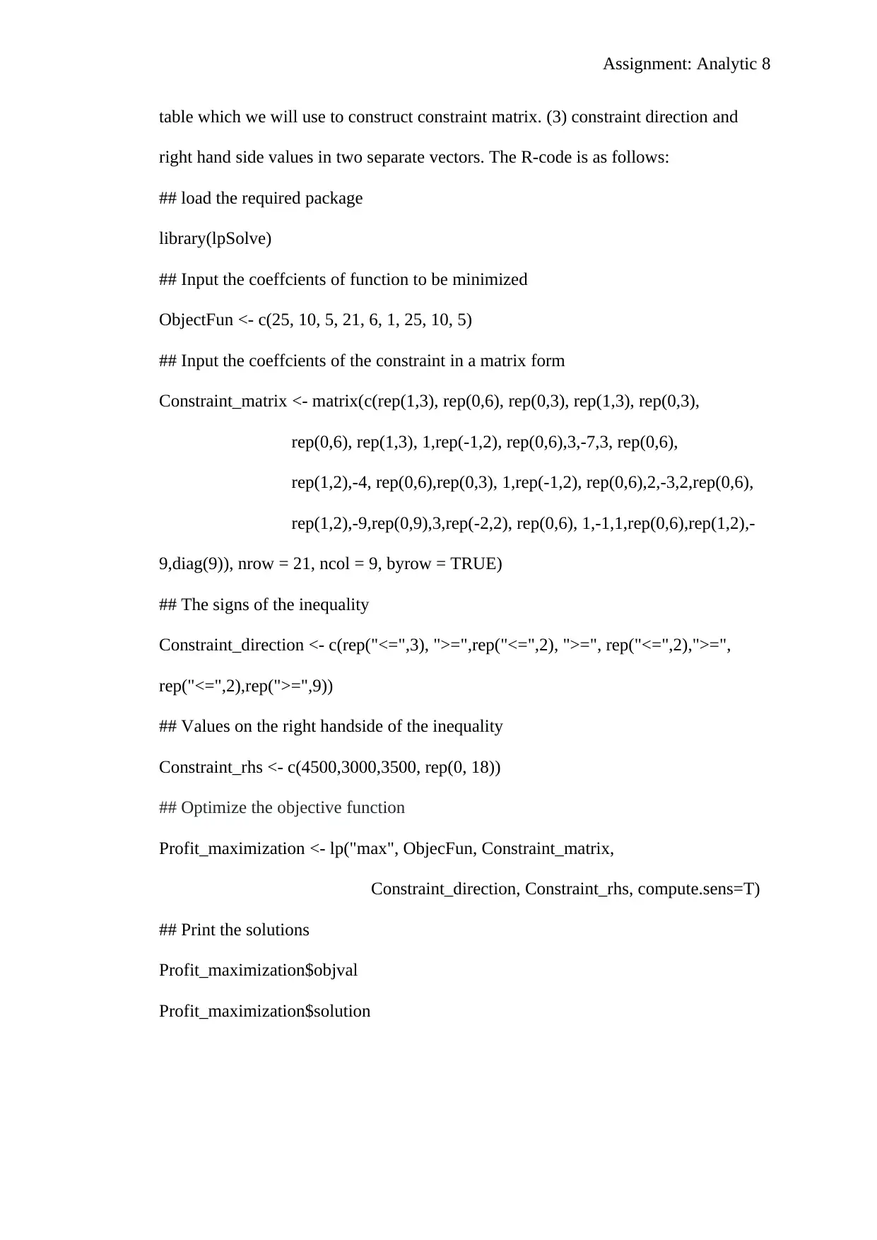
(b) The lpSolve parckage in R-studio was used. In specifict the lp function was used. The
function require four main inputs: (1) coefficients of the decision variables in the
objective function as a vectors (Akpinar and Baykasoglu 2014; Recht, Re and Bittorf
2012). (2) coeffcients of the decision variables as a n x m matrix thing is to make a
xs 3
xc3 +xw 3+ xs 3
≥ 0.1 ⟺ xc 3+xw 3−9 x s3 ≤ 0
The certainity constraints
xc 1 ≥ 0 , xc 2 ≥ 0 , xc3 ≥ 0 , xs 1 ≥ 0 , xs 2 ≥0 , xs 3 ≥0 , xw 1 ≥ 0 , xw2 ≥ 0 , xw 3 ≥0
Therefore, the LP problem is to maximize profit subject to demand, prorportion of
material in each product and certainity constraints. That is
Max P=25 xc 1+10 xw 1 +5 xs 1+21 xc2 +6 xw 2 + xs 2+ 25 xc 3 +10 xw3 +5 xs 3 Subject to:
xc 1+xw 1 + xs 1 ≤ 4500
xc 2+ xw 2 +xs 2 ≤ 3000
xc 3+xw 3 + xs 3 ≤3500
xc 1−xw1 −xs 1 ≥ 0
3 xc1−7 xw 1 +3 xs 1 ≤ 0
xc 1+ xw 1−4 xs 1 ≤ 0
xc 2−xw 2−xs 2 ≥ 0
2 xc2−3 xw 2 +2 xs 2 ≤ 0
xc 2+ xw 2−9 xs 2 ≤ 0
3 xc3 −2 xw 3−2 xs 3 ≥ 0
xc 3−xw 3+ x s3 ≤ 0
xc 3+xw 3−9 x s3 ≤ 0
xij ≥ 0
(b) The lpSolve parckage in R-studio was used. In specifict the lp function was used. The
function require four main inputs: (1) coefficients of the decision variables in the
objective function as a vectors (Akpinar and Baykasoglu 2014; Recht, Re and Bittorf
2012). (2) coeffcients of the decision variables as a n x m matrix thing is to make a
Paraphrase This Document
Need a fresh take? Get an instant paraphrase of this document with our AI Paraphraser
Assignment: Analytic 8
table which we will use to construct constraint matrix. (3) constraint direction and
right hand side values in two separate vectors. The R-code is as follows:
## load the required package
library(lpSolve)
## Input the coeffcients of function to be minimized
ObjectFun <- c(25, 10, 5, 21, 6, 1, 25, 10, 5)
## Input the coeffcients of the constraint in a matrix form
Constraint_matrix <- matrix(c(rep(1,3), rep(0,6), rep(0,3), rep(1,3), rep(0,3),
rep(0,6), rep(1,3), 1,rep(-1,2), rep(0,6),3,-7,3, rep(0,6),
rep(1,2),-4, rep(0,6),rep(0,3), 1,rep(-1,2), rep(0,6),2,-3,2,rep(0,6),
rep(1,2),-9,rep(0,9),3,rep(-2,2), rep(0,6), 1,-1,1,rep(0,6),rep(1,2),-
9,diag(9)), nrow = 21, ncol = 9, byrow = TRUE)
## The signs of the inequality
Constraint_direction <- c(rep("<=",3), ">=",rep("<=",2), ">=", rep("<=",2),">=",
rep("<=",2),rep(">=",9))
## Values on the right handside of the inequality
Constraint_rhs <- c(4500,3000,3500, rep(0, 18))
## Optimize the objective function
Profit_maximization <- lp("max", ObjecFun, Constraint_matrix,
Constraint_direction, Constraint_rhs, compute.sens=T)
## Print the solutions
Profit_maximization$objval
Profit_maximization$solution
Assignment: Analytic 9
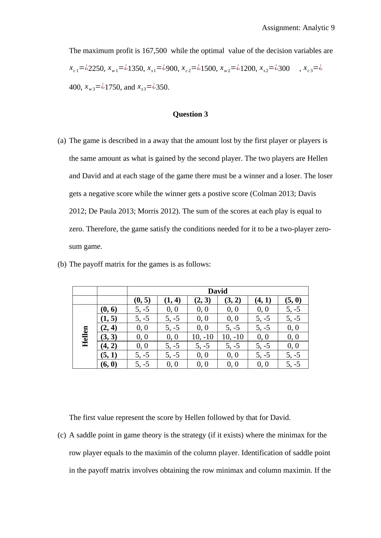
The maximum profit is 167,500 while the optimal value of the decision variables are
xc 1=¿2250, xw 1=¿1350, xs 1=¿900, xc 2=¿1500, xw 2=¿1200, xs 2=¿300 , xc 3=¿
400, xw 3=¿1750, and xs 3=¿350.
Question 3
(a) The game is described in a away that the amount lost by the first player or players is
the same amount as what is gained by the second player. The two players are Hellen
and David and at each stage of the game there must be a winner and a loser. The loser
gets a negative score while the winner gets a postive score (Colman 2013; Davis
2012; De Paula 2013; Morris 2012). The sum of the scores at each play is equal to
zero. Therefore, the game satisfy the conditions needed for it to be a two-player zero-
sum game.
(b) The payoff matrix for the games is as follows:
David
(0, 5) (1, 4) (2, 3) (3, 2) (4, 1) (5, 0)
Hellen
(0, 6) 5, -5 0, 0 0, 0 0, 0 0, 0 5, -5
(1, 5) 5, -5 5, -5 0, 0 0, 0 5, -5 5, -5
(2, 4) 0, 0 5, -5 0, 0 5, -5 5, -5 0, 0
(3, 3) 0, 0 0, 0 10, -10 10, -10 0, 0 0, 0
(4, 2) 0, 0 5, -5 5, -5 5, -5 5, -5 0, 0
(5, 1) 5, -5 5, -5 0, 0 0, 0 5, -5 5, -5
(6, 0) 5, -5 0, 0 0, 0 0, 0 0, 0 5, -5
The first value represent the score by Hellen followed by that for David.
(c) A saddle point in game theory is the strategy (if it exists) where the minimax for the
row player equals to the maximin of the column player. Identification of saddle point
in the payoff matrix involves obtaining the row minimax and column maximin. If the
⊘ This is a preview!⊘
Do you want full access?
Subscribe today to unlock all pages.
Trusted by 1+ million students worldwide
Assignment: Analytic 10
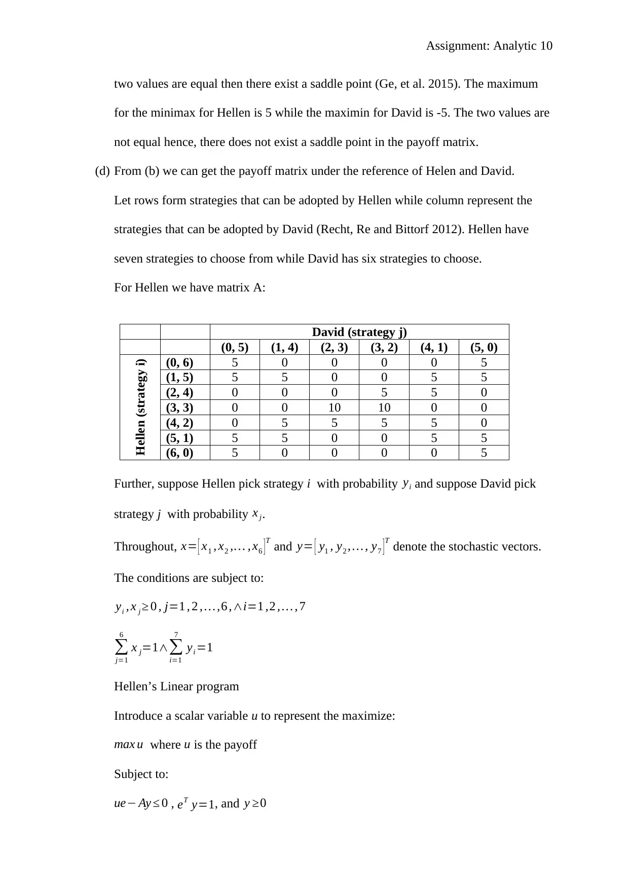
two values are equal then there exist a saddle point (Ge, et al. 2015). The maximum
for the minimax for Hellen is 5 while the maximin for David is -5. The two values are
not equal hence, there does not exist a saddle point in the payoff matrix.
(d) From (b) we can get the payoff matrix under the reference of Helen and David.
Let rows form strategies that can be adopted by Hellen while column represent the
strategies that can be adopted by David (Recht, Re and Bittorf 2012). Hellen have
seven strategies to choose from while David has six strategies to choose.
For Hellen we have matrix A:
David (strategy j)
(0, 5) (1, 4) (2, 3) (3, 2) (4, 1) (5, 0)
Hellen (strategy i) (0, 6) 5 0 0 0 0 5
(1, 5) 5 5 0 0 5 5
(2, 4) 0 0 0 5 5 0
(3, 3) 0 0 10 10 0 0
(4, 2) 0 5 5 5 5 0
(5, 1) 5 5 0 0 5 5
(6, 0) 5 0 0 0 0 5
Further, suppose Hellen pick strategy i with probability yi and suppose David pick
strategy j with probability x j.
Throughout, x= [ x1 , x2 ,… , x6 ]T and y= [ y1 , y2 , … , y7 ]T denote the stochastic vectors.
The conditions are subject to:
yi , x j ≥ 0 , j=1 , 2 , … ,6 ,∧i=1 ,2 , … , 7
∑
j=1
6
x j=1∧∑
i=1
7
yi =1
Hellen’s Linear program
Introduce a scalar variable u to represent the maximize:
max u where u is the payoff
Subject to:
ue− Ay ≤ 0 , eT y=1, and y ≥0
Paraphrase This Document
Need a fresh take? Get an instant paraphrase of this document with our AI Paraphraser
Assignment: Analytic 11
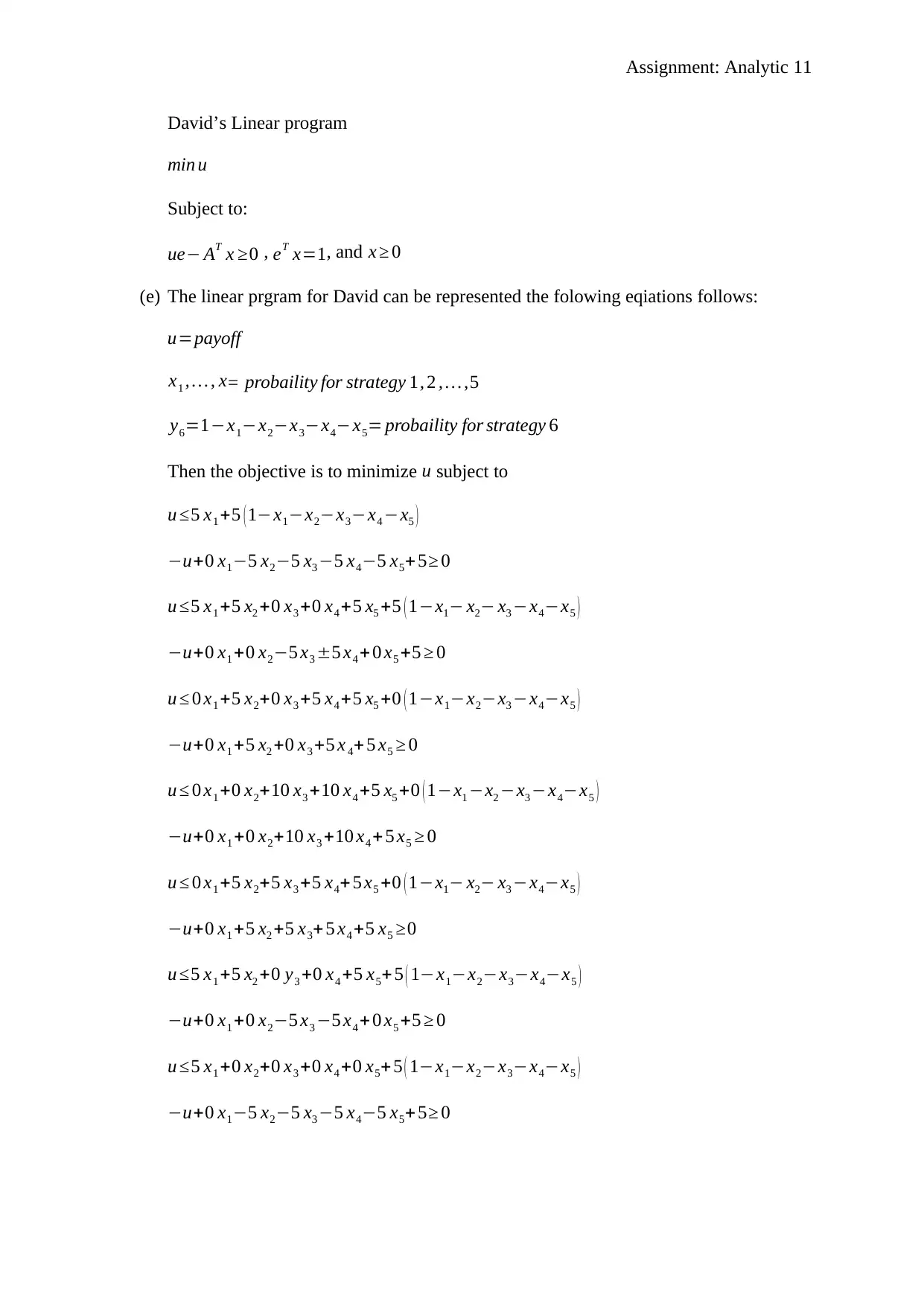
David’s Linear program
min u
Subject to:
ue− AT x ≥0 , eT x=1, and x ≥ 0
(e) The linear prgram for David can be represented the folowing eqiations follows:
u=payoff
x1 , … , x= probaility for strategy 1, 2 , … ,5
y6=1−x1−x2−x3−x4−x5= probaility for strategy 6
Then the objective is to minimize u subject to
u ≤5 x1 +5 ( 1−x1−x2−x3−x4 −x5 )
−u+0 x1−5 x2−5 x3 −5 x4−5 x5+ 5≥ 0
u ≤5 x1 +5 x2 +0 x3 +0 x4 +5 x5 +5 ( 1−x1− x2− x3 −x4−x5 )
−u+0 x1 +0 x2−5 x3 ±5 x4 + 0 x5 +5 ≥ 0
u ≤ 0 x1 +5 x2+0 x3 +5 x4 +5 x5 +0 ( 1−x1−x2−x3 −x4−x5 )
−u+0 x1 +5 x2 +0 x3 +5 x 4+ 5 x5 ≥ 0
u ≤ 0 x1 +0 x2+10 x3 +10 x4 +5 x5 +0 ( 1−x1 −x2 −x3 −x4−x5 )
−u+0 x1 +0 x2+10 x3 +10 x4 +5 x5 ≥ 0
u ≤ 0 x1 +5 x2+5 x3 +5 x4+ 5 x5 +0 ( 1−x1− x2− x3 −x4−x5 )
−u+0 x1 +5 x2 +5 x3+ 5 x4 +5 x5 ≥0
u ≤5 x1 +5 x2 +0 y3 +0 x4 +5 x5+ 5 ( 1−x1−x2−x3−x4−x5 )
−u+0 x1 +0 x2−5 x3 −5 x4 + 0 x5 +5 ≥ 0
u ≤5 x1 +0 x2+0 x3 +0 x4 +0 x5+ 5 ( 1−x1−x2−x3−x4−x5 )
−u+0 x1−5 x2−5 x3 −5 x4−5 x5+ 5≥ 0
Assignment: Analytic 12
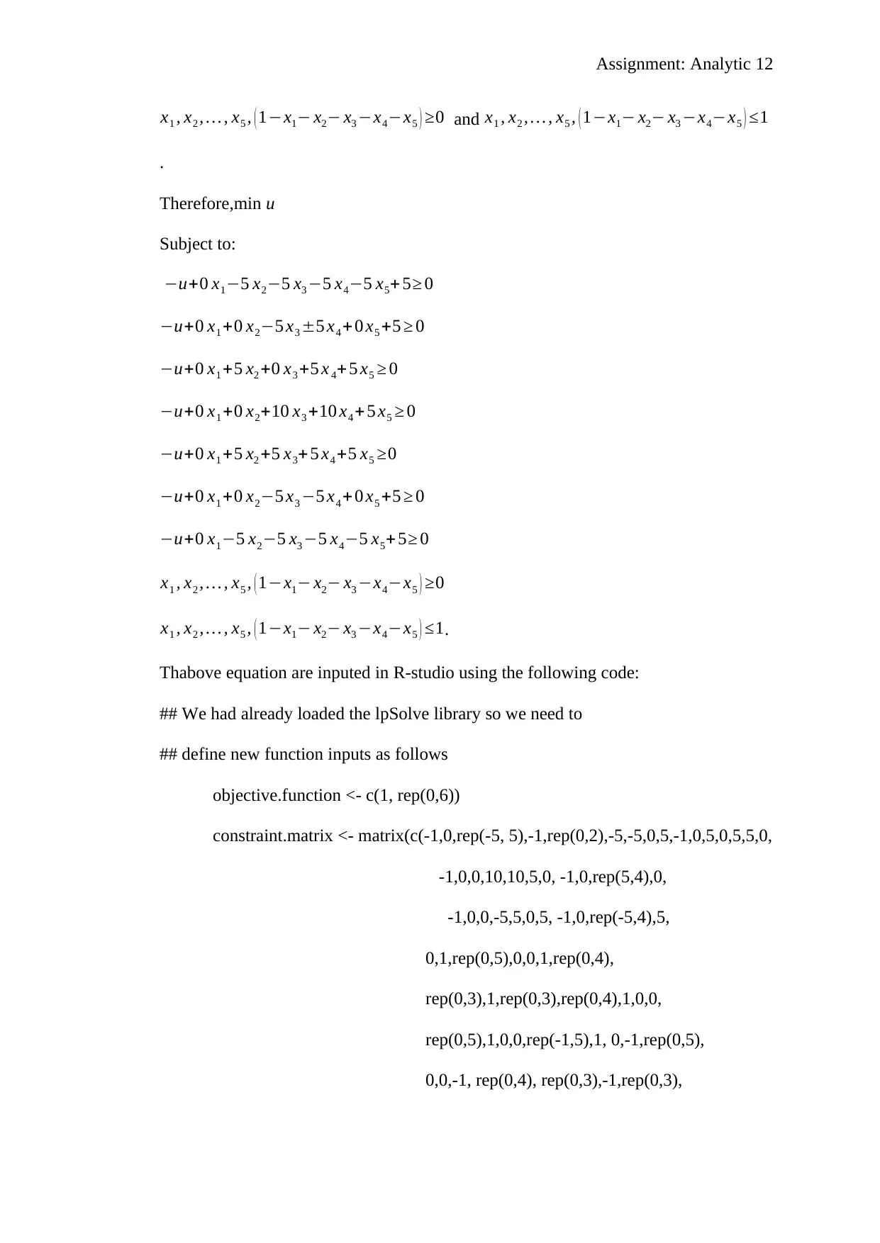
x1 , x2 , … , x5 , ( 1−x1− x2− x3 −x4−x5 ) ≥0 and x1 , x2 , … , x5 , ( 1−x1− x2− x3 −x4−x5 ) ≤1
.
Therefore,min u
Subject to:
−u+0 x1−5 x2−5 x3 −5 x4−5 x5+ 5≥ 0
−u+0 x1 +0 x2−5 x3 ±5 x4 + 0 x5 +5 ≥ 0
−u+0 x1 +5 x2 +0 x3 +5 x 4+ 5 x5 ≥ 0
−u+0 x1 +0 x2+10 x3 +10 x4 +5 x5 ≥ 0
−u+0 x1 +5 x2 +5 x3+ 5 x4 +5 x5 ≥0
−u+0 x1 +0 x2−5 x3 −5 x4 + 0 x5 +5 ≥ 0
−u+0 x1−5 x2−5 x3 −5 x4−5 x5+ 5≥ 0
x1 , x2 , … , x5 , ( 1−x1− x2− x3 −x4−x5 ) ≥0
x1 , x2 , … , x5 , ( 1−x1− x2− x3 −x4−x5 ) ≤1.
Thabove equation are inputed in R-studio using the following code:
## We had already loaded the lpSolve library so we need to
## define new function inputs as follows
objective.function <- c(1, rep(0,6))
constraint.matrix <- matrix(c(-1,0,rep(-5, 5),-1,rep(0,2),-5,-5,0,5,-1,0,5,0,5,5,0,
-1,0,0,10,10,5,0, -1,0,rep(5,4),0,
-1,0,0,-5,5,0,5, -1,0,rep(-5,4),5,
0,1,rep(0,5),0,0,1,rep(0,4),
rep(0,3),1,rep(0,3),rep(0,4),1,0,0,
rep(0,5),1,0,0,rep(-1,5),1, 0,-1,rep(0,5),
0,0,-1, rep(0,4), rep(0,3),-1,rep(0,3),
⊘ This is a preview!⊘
Do you want full access?
Subscribe today to unlock all pages.
Trusted by 1+ million students worldwide
1 out of 17
Related Documents


![Course Name: Real World Analytics Assignment Solution - [Date]](/_next/image/?url=https%3A%2F%2Fdesklib.com%2Fmedia%2Fimages%2Fjs%2F7cd677b2bca5453d86bfbb121190a9b2.jpg&w=256&q=75)

Your All-in-One AI-Powered Toolkit for Academic Success.
+13062052269
info@desklib.com
Available 24*7 on WhatsApp / Email
![[object Object]](/_next/static/media/star-bottom.7253800d.svg)
Unlock your academic potential
Copyright © 2020–2026 A2Z Services. All Rights Reserved. Developed and managed by ZUCOL.