SIT718 Real World Analytics Assignment: Problem Solving Solution

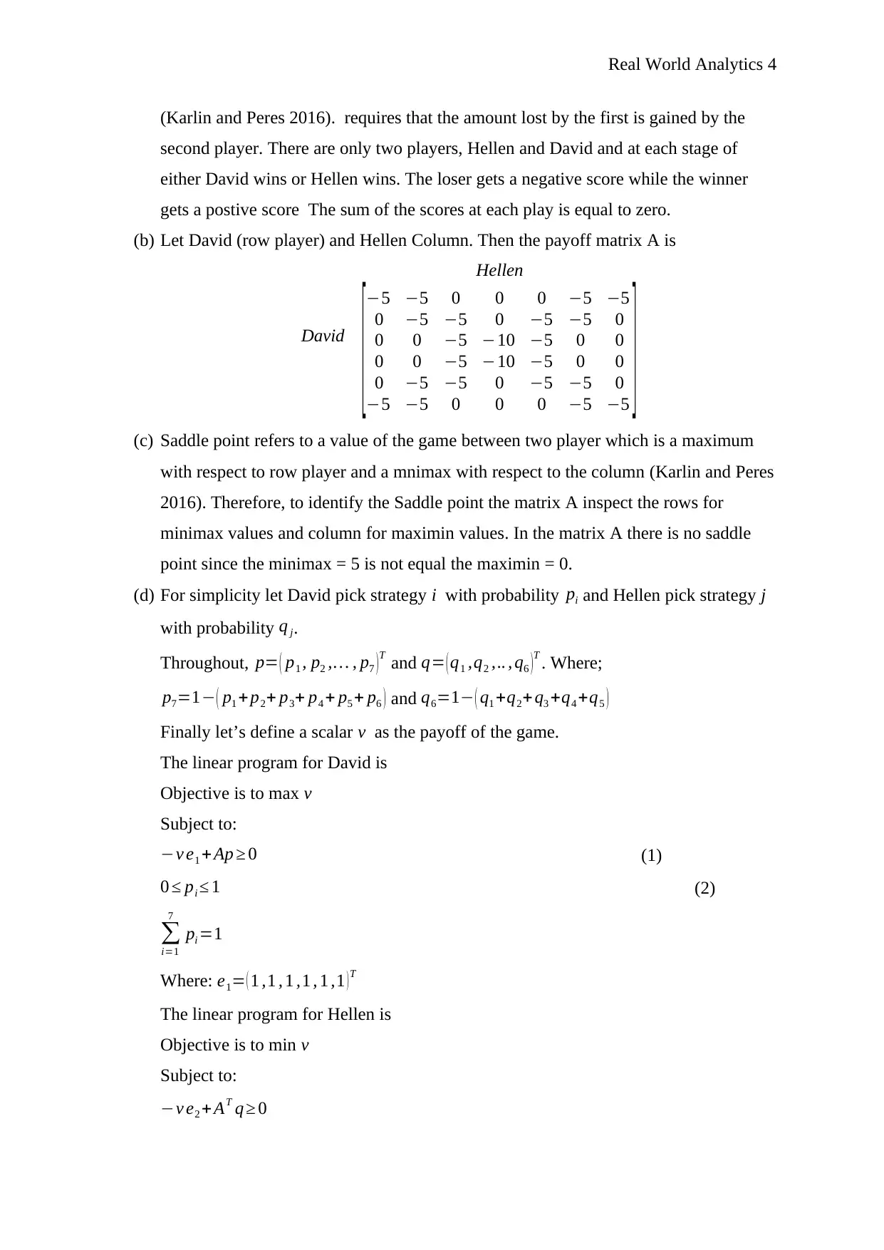
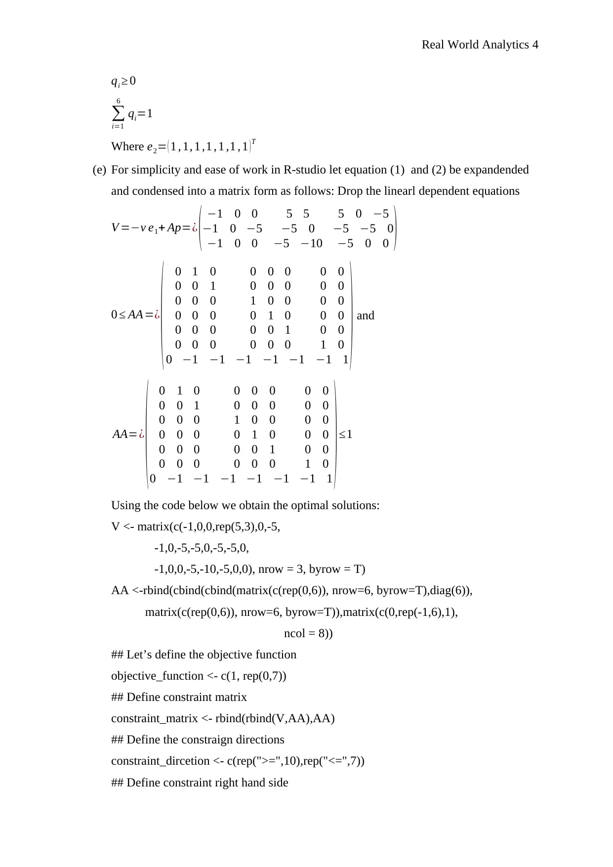
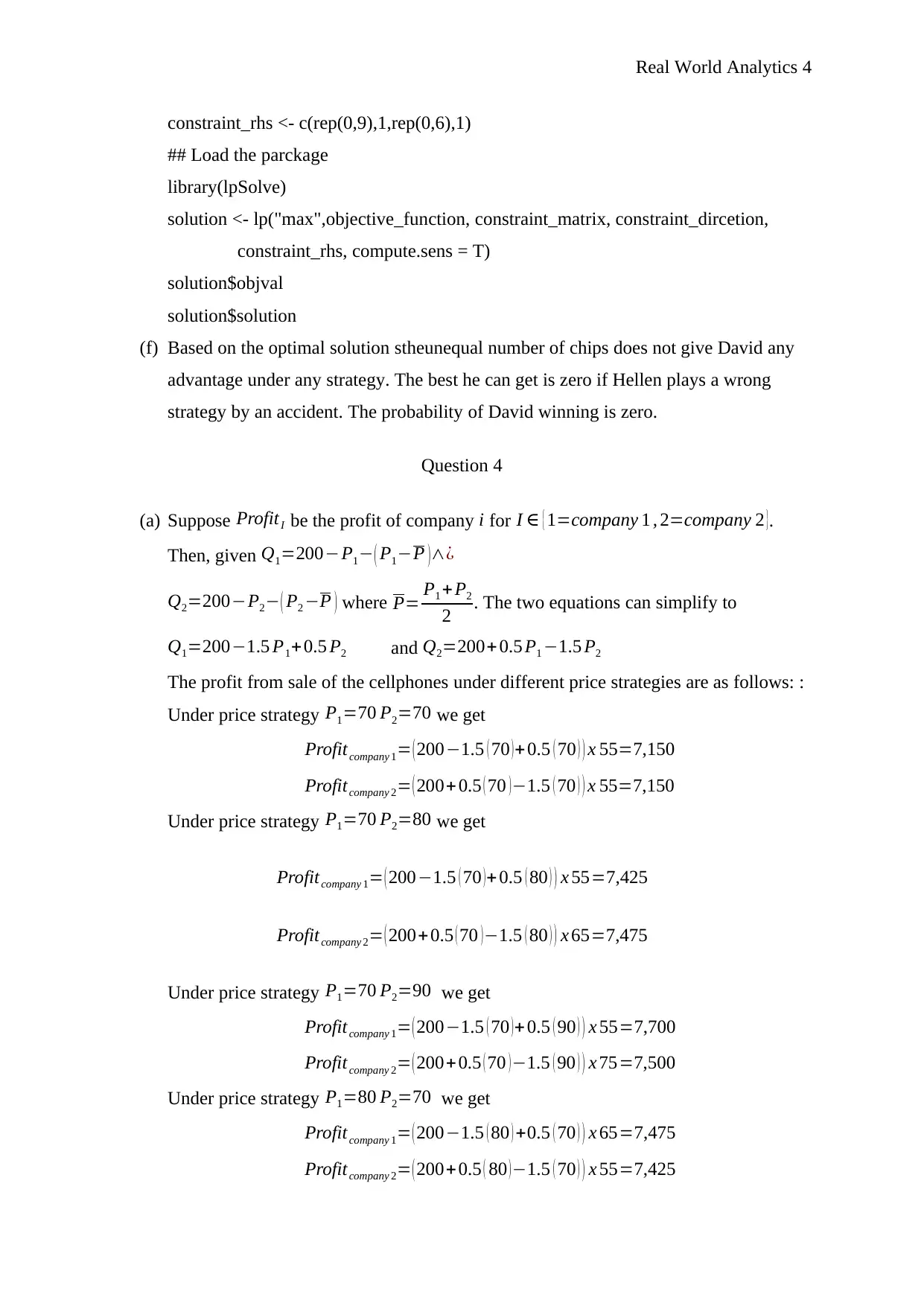
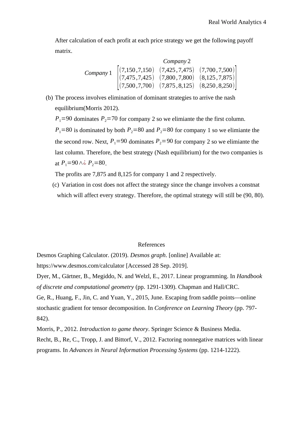
This document presents a comprehensive solution to a Real World Analytics assignment, addressing problems using linear programming and game theory. The solution includes detailed explanations and mathematical formulations for optimizing costs in beverage production (Question 1), maximizing profit in product manufacturing (Question 2), analyzing zero-sum games (Question 3), and determining Nash equilibrium in pricing strategies (Question 4). The assignment utilizes graphical methods, linear programming solvers, and R code to arrive at optimal decisions, demonstrating the application of analytical techniques to real-world scenarios. The solution covers topics such as constraint optimization, decision variables, payoff matrices, and the identification of saddle points and Nash equilibrium.

Real World Analytics 4
Real World Analytics
by[Name]
Course
Professor’s Name
Institution
Location of Institution
Date

Real World Analytics 4
Real World Analytics
Question 1
(a) The problem can be presented in form of a set of linear equations. There is an
objective in the problem (minimize costs) and the function has a direct linear
relationship with the restrictions on the mount of product A or B than can be used in
making the beverage (Morris 2012). The other condition that the problem satisfy is
the non-negativity assumption of linear programming. Since we cannot use less than
zero units of the ingredients in making the beverage. Therefore, the problem can be
modeled by a linear programming method.
(b) In order to represent the problem in mathematical terms, let the food factory use x =
liters of product A and y liters of product B in producing the beverage. This implies
that the total volume of beverage produced is (x + y) liters.
C = 5x + 7y.
In addition to the cost the restrictions are presented as follows:
Orange Mango Lime
x + 2
3 y ≥ 75, x + 3
2 y ≥ 125, x + 8
3 y ≤2 00
Certainty constraint: x ≥ 0 and y≥ 0.
In mathematical terms, the problem is to:
Min C = 5x + 7y.
Subject to:
x + 2
3 y ≥ 75, x + 3
2 y ≥ 125, x + 8
3 y ≤2 00, x ≥ 0 and y≥ 0.
(c) The equation is plotted in desmos.com as shown in screenshot below

Real World Analytics 4
Using the values at the corner points gives a minimum total cost of 595 at point (35,
60). Therefore, the factory should use 35 liters of product A and 60 liters of product B
to produce 95 liters of the beaverage.
(d) If we increase the liters of A by one unit the new optimal solution is at point (33.33,
62.5). This means that the price should be less than one. After tring values between 5
to 5.9 we realise the values that A can take without chnaging the position of the
optimal solution is between 5 and 5.85 liters of product A.
Question 2
(a) Given xij ≥ 0 is the decision variable that denotes the number of tons of products j for
j ϵ { 1=Spring;2=Autumn ; 3=Winter } to be produced from materials i for
i ϵ {C=Cotton ,W =Wool , S=Silk } . Also, the proportion of a particular type of
material in a particular type of product can be calculated as xc1
xc1 + xw 1+ xs 1
proportion
of cotton in Spring. Let profit be the difference between total cost and the total
revenue, given as:
Profit = Cost – Revenue, where Cost = production cost + purcahse cost, Revenue =
sales price x deamnd. Then,
Revenue=60 xc1 +60 xw 1+60 xs 1 +55 xc2 +55 xw 2+55 xs 2 +60 xc3 +60 xw 3+60 x s3
Production cost=5 ( xc 1+ xw1 +xs 1 ) +4 ( xc2 +xw 2+ xs 2 )+ 5 ( xc3 + xw 3+ xs 3 )
Purchase cost=30 xc1 + 45 xw 1 +50 xs 1+30 xc 2+ 45 xw 2+50 xs 2 +30 xc3 + 45 xw 3 +50 xs 3
Cost =35 xc 1 +50 xw1 +55 xs 1+ 34 xc2 + 49 xw 2 +54 xs 2 +35 xc3 +50 xw3 +55 xs 3
Profit=25 xc1 +10 xw 1+5 xs 1 +21 xc 2 +6 xw 2+x s2 +25 xc 3+10 xw 3 +5 xs 3
Therefore, we

Real World Analytics 4
Max Profit=25 xc1 +10 xw 1+5 xs 1 +21 xc 2 +6 xw 2+ x s2 +25 xc 3+10 xw 3 +5 xs 3 Subject to:
xc 1+xw 1 + xs 1 ≤ 4500 , xc 2+ xw 2 +xs 2 ≤ 3000, xc 3+ xw 3 + xs 3 ≤3500, xc 1−xw1 −xs 1 ≥ 0,
3 xc1−7 xw 1 +3 xs 1 ≤ 0, xc 1+ xw 1−4 xs 1 ≤ 0, xc 2−xw 2−xs 2 ≥ 0, 2 xc2−3 xw 2 +2 xs 2 ≤ 0,
xc 2+ xw 2−9 xs 2 ≤ 0
3 xc3 −2 xw 3−2 xs 3 ≥ 0, xc 3−xw 3+ x s3 ≤ 0, xc 3+ xw 3−9 x s3 ≤ 0
And the non-negativity constraints:
xc 1 ≥ 0 , xc 2 ≥ 0 , xc3 ≥ 0 , xs 1 ≥ 0 , xs 2 ≥0 , xs 3 ≥0 , xw 1 ≥ 0 , xw2 ≥ 0 , xw 3 ≥0.
(b) The R-code is as follows:
library(lpSolve)
ObjecFunction <- c(25, 10, 5, 21, 6, 1, 25, 10, 5)
ConstraintMatrix <- matrix(c(rep(1,3), rep(0,6),
rep(0,3), rep(1,3), rep(0,3),
rep(0,6), rep(1,3),
1,-1,-1, rep(0,6),3,-7,3, rep(0,6),
1,1,-4, rep(0,6),rep(0,3),
1,-1,-1, rep(0,6),2,-3,2,rep(0,6),
1,1,-9,rep(0,9),3,-2,-2, rep(0,6),
1,-1,1,rep(0,6),1,1,-9,diag(9)),
nrow = 21, ncol = 9, byrow = TRUE)
ConstraintDirection <- c(rep("<=",3), ">=",rep("<=",2),
">=",rep("<=",2),">=",rep("<=",2),rep(">=",9))
ConstraintRhs <- c(4500,3000,3500, rep(0, 18))
Optimize <- lp("max", ObjecFunction, ConstraintMatrix,
ConstraintDirection, ConstraintRhs, compute.sens=T)
Optimize$objval
Optimize$solution
The maximum profit is $167,500 while the optimal value of the decision variables
are xc 1=¿2250, xw 1=¿1350, xs 1=¿900, xc 2=¿1500, xw 2=¿1200, xs 2=¿300 ,
xc 3=1400, xw 3=¿1750, and xs 3=¿350.
Question 3
(a) The description of the games satisfies the conditions for a zeros sum game as follows:
There does not exist more than one win or loss for each player at each turn of the play

Real World Analytics 4
(Karlin and Peres 2016). requires that the amount lost by the first is gained by the
second player. There are only two players, Hellen and David and at each stage of
either David wins or Hellen wins. The loser gets a negative score while the winner
gets a postive score The sum of the scores at each play is equal to zero.
(b) Let David (row player) and Hellen Column. Then the payoff matrix A is
David
Hellen
[−5
0
0
−5 0 0
−5 −5 0
0 −5 −10
0 −5 −5
−5 −5 0
−5 0 0
0
0
−5
0 −5 −10
−5 −5 0
−5 0 0
−5 0 0
−5 −5 0
0 −5 −5
](c) Saddle point refers to a value of the game between two player which is a maximum
with respect to row player and a mnimax with respect to the column (Karlin and Peres
2016). Therefore, to identify the Saddle point the matrix A inspect the rows for
minimax values and column for maximin values. In the matrix A there is no saddle
point since the minimax = 5 is not equal the maximin = 0.
(d) For simplicity let David pick strategy i with probability pi and Hellen pick strategy j
with probability q j.
Throughout, p= ( p1 , p2 ,… , p7 )T and q= ( q1 ,q2 ,.. , q6 )T . Where;
p7=1− ( p1 +p2+ p3+ p4 + p5 + p6 ) and q6=1− ( q1 +q2+ q3 +q4 +q5 )
Finally let’s define a scalar v as the payoff of the game.
The linear program for David is
Objective is to max v
Subject to:
−v e1 +Ap ≥ 0 (1)
0 ≤ pi ≤ 1 (2)
∑
i=1
7
pi =1
Where: e1= ( 1 ,1 , 1 ,1 , 1 ,1 ) T
The linear program for Hellen is
Objective is to min v
Subject to:
−v e2 +AT q ≥ 0

Real World Analytics 4
qi ≥ 0
∑
i=1
6
qi=1
Where e2= ( 1 , 1, 1 ,1 , 1 ,1 , 1 ) T
(e) For simplicity and ease of work in R-studio let equation (1) and (2) be expandended
and condensed into a matrix form as follows: Drop the linearl dependent equations
V =−v e1+ Ap=¿ ( −1 0 0 5 5 5 0 −5
−1 0 −5 −5 0 −5 −5 0
−1 0 0 −5 −10 −5 0 0 )
0 ≤ AA=¿
( 0 1 0
0 0 1
0 0 0
0 0 0
0 0 0
1 0 0
0 0
0 0
0 0
0 0 0
0 0 0
0 0 0
0 1 0
0 0 1
0 0 0
0 0
0 0
1 0
0 −1 −1 −1 −1 −1 −1 1
) and
AA=¿
( 0 1 0
0 0 1
0 0 0
0 0 0
0 0 0
1 0 0
0 0
0 0
0 0
0 0 0
0 0 0
0 0 0
0 1 0
0 0 1
0 0 0
0 0
0 0
1 0
0 −1 −1 −1 −1 −1 −1 1
)≤1
Using the code below we obtain the optimal solutions:
V <- matrix(c(-1,0,0,rep(5,3),0,-5,
-1,0,-5,-5,0,-5,-5,0,
-1,0,0,-5,-10,-5,0,0), nrow = 3, byrow = T)
AA <-rbind(cbind(cbind(matrix(c(rep(0,6)), nrow=6, byrow=T),diag(6)),
matrix(c(rep(0,6)), nrow=6, byrow=T)),matrix(c(0,rep(-1,6),1),
ncol = 8))
## Let’s define the objective function
objective_function <- c(1, rep(0,7))
## Define constraint matrix
constraint_matrix <- rbind(rbind(V,AA),AA)
## Define the constraign directions
constraint_dircetion <- c(rep(">=",10),rep("<=",7))
## Define constraint right hand side

Real World Analytics 4
constraint_rhs <- c(rep(0,9),1,rep(0,6),1)
## Load the parckage
library(lpSolve)
solution <- lp("max",objective_function, constraint_matrix, constraint_dircetion,
constraint_rhs, compute.sens = T)
solution$objval
solution$solution
(f) Based on the optimal solution stheunequal number of chips does not give David any
advantage under any strategy. The best he can get is zero if Hellen plays a wrong
strategy by an accident. The probability of David winning is zero.
Question 4
(a) Suppose ProfitI be the profit of company i for I ∈ { 1=company 1 , 2=company 2 }.
Then, given Q1=200−P1− ( P1−P )∧¿
Q2=200−P2− ( P2 −P ) where P= P1 +P2
2 . The two equations can simplify to
Q1=200−1.5 P1+0.5 P2 and Q2=200+ 0.5 P1 −1.5 P2
The profit from sale of the cellphones under different price strategies are as follows: :
Under price strategy P1=70 P2=70 we get
Profitcompany 1= ( 200−1.5 ( 70 )+0.5 ( 70 ) ) x 55=7,150
Profitcompany 2= ( 200+0.5 ( 70 ) −1.5 ( 70 ) ) x 55=7,150
Under price strategy P1=70 P2=80 we get
Profitcompany 1= ( 200−1.5 ( 70 ) + 0.5 ( 80 ) ) x 55=7,425
Profitcompany 2= ( 200+ 0.5 ( 70 ) −1.5 ( 80 ) ) x 65=7,475
Under price strategy P1=70 P2=90 we get
Profitcompany 1= ( 200−1.5 ( 70 )+ 0.5 ( 90 ) ) x 55=7,700
Profitcompany 2= ( 200+0.5 ( 70 ) −1.5 ( 90 ) ) x 75=7,500
Under price strategy P1=80 P2=70 we get
Profitcompany 1= ( 200−1.5 ( 80 ) +0.5 ( 70 ) ) x 65=7,475
Profitcompany 2= ( 200+ 0.5 ( 80 )−1.5 ( 70 ) ) x 55=7,425

Real World Analytics 4
After calculation of each profit at each price strategy we get the following payoff
matrix.
Company 1
Company 2
[ (7,150 ,7,150) (7,425 , 7,475) (7,700 , 7,500)
(7,475 ,7,425) (7,800 , 7,800) (8,125 , 7,875)
(7,500 ,7,700) (7,875 , 8,125) (8,250 , 8,250) ]
(b) The process involves elimination of dominant strategies to arrive the nash
equilibrium(Morris 2012).
P1=90 dominates P2=70 for company 2 so we elimiante the the first column.
P1=80 is dominated by both P2=80 and P2=80 for company 1 so we elimiante the
the second row. Next, P1=90 dominates P2=90 for company 2 so we elimiante the
last column. Therefore, the best strategy (Nash equilibrium) for the two companies is
at P1=90∧¿ P2=80.
The profits are 7,875 and 8,125 for company 1 and 2 respectively.
(c) Variation in cost does not affect the strategy since the change involves a constnat
which will affect every strategy. Therefore, the optimal strategy will still be (90, 80).
References
Desmos Graphing Calculator. (2019). Desmos graph. [online] Available at:
https://www.desmos.com/calculator [Accessed 28 Sep. 2019].
Dyer, M., Gärtner, B., Megiddo, N. and Welzl, E., 2017. Linear programming. In Handbook
of discrete and computational geometry (pp. 1291-1309). Chapman and Hall/CRC.
Ge, R., Huang, F., Jin, C. and Yuan, Y., 2015, June. Escaping from saddle points—online
stochastic gradient for tensor decomposition. In Conference on Learning Theory (pp. 797-
842).
Morris, P., 2012. Introduction to game theory. Springer Science & Business Media.
Recht, B., Re, C., Tropp, J. and Bittorf, V., 2012. Factoring nonnegative matrices with linear
programs. In Advances in Neural Information Processing Systems (pp. 1214-1222).