SIT718 Real World Analytics: Stock Price Prediction using R - ANZ

This report delves into the stock price analysis of Australia and New Zealand (ANZ) Banking Group, a major international financial institution. It utilizes R statistical package to explore and visualize stock price trends over a three-month period, employing stochastic modeling techniques, particularly Geometric Brownian Motion (GBM), to estimate and predict price movements. The analysis includes the computation of key parameters such as volatility and drift, examining their impact on stock prices. The report also assesses the normality property of the stock prices, crucial for GBM applicability, and estimates expected stock values, comparing them with actual published data. The study concludes by highlighting the factors influencing stock price instability and emphasizing the effectiveness of stochastic modeling in capturing these dynamics. It also provides the R code used for the analysis.

Running header: Analytics 1
Read World Analytics
Name:
Course title:
Instructor:
Date:

Analytics 2
1. Australia and New Zealand (ANZ) Banking Group
Among various companies, Australia and New Zealand (ANZ) Banking group is one of the
biggest international banking and financial services group across the globe. Moreover, it is the largest
company in New Zealand following the acquisition of The National Bank of New Zealand in 2003.
Notably, ANZ was initiated in 1830 as the Bank of Australia to become Australia’s leading and fastest
developing bank. The company has its branches across the two countries; however, the headquarter is
located in Melbourne, Australia. The company has experienced tremendous growth in the past two
decades, which resulted in its listing in various stock exchange platforms, such as New Zealand, and
Australia. The company offers multiple services to its customers, which include banking, investment, and
insurance, among others. Therefore, the study seeks to explore the changes exhibited by the stock prices
of AZN; moreover, R statistical package will be used to predict the stock prices and compute factors
affecting the prices.
2. Data exploration and visualization
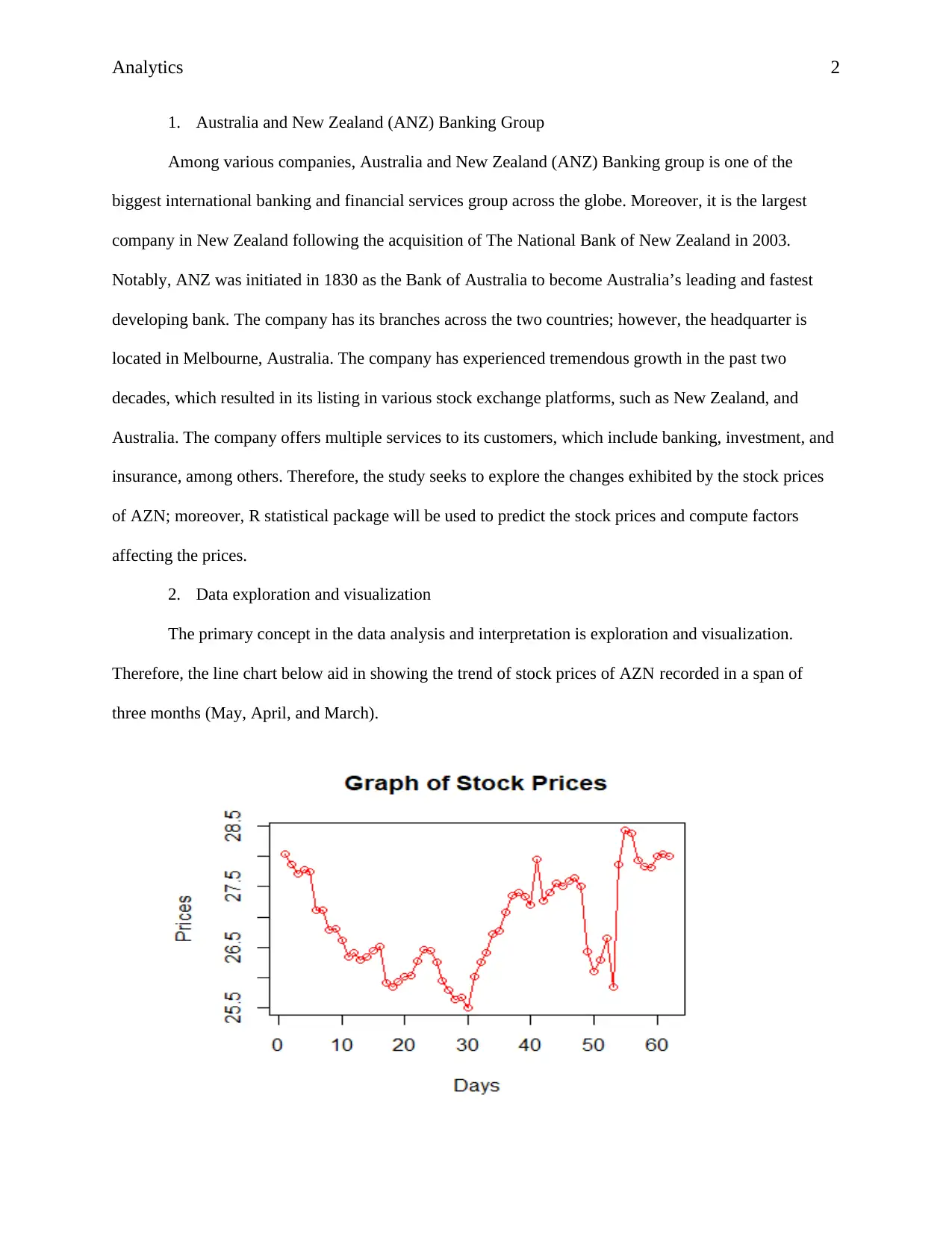
The primary concept in the data analysis and interpretation is exploration and visualization.
Therefore, the line chart below aid in showing the trend of stock prices of AZN recorded in a span of
three months (May, April, and March).

Analytics 3
3. Stochastic Modelling
There is no doubt one of the highly volatile variables in stock exchange markets is the stock
price. As a result, the variable possesses the unstable property caused by various factors, such as liquidity
on stock return, which result in the random and frequent changes or shifts in the prices (Adeosun, et al.,
2015, 353). As a result, various stakeholders, such as investors, co-operations, and researchers, among
others, tend to look for convenient techniques to estimate or predict the expected movement in the prices.
Among various methods used in the estimation of share prices, the stochastic modelling is the most
effective and suitable technique since the unstable property of the variable assumes a Markov process (a
primal component of stochastic modelling) (Antwi, 2017, 116). Consequently, Geometric Brownian
Motion the most applicable stochastic model used in the estimation of stock prices. The GBM model is
derived from the Brownian Motion (BM) developed by Robert Brown to explain the haphazard
movements of particles due to collision (Adeosun, et al., 2015, 353). Notably, unlike BM, the GBM only
takes values greater than zero (positive values); thus, it is an effective model (Imperial, 2018, 3). The
following function exhibits the GBM model;
S(t) = S0 exp W(t)
Whereby W(t) = μ + σ2/2
S0 is the initial stock price
S(t) is the current stock price (t)
μ represent the drift in a stochastic process
σ represent the volatility in a stochastic process
i. Volatility
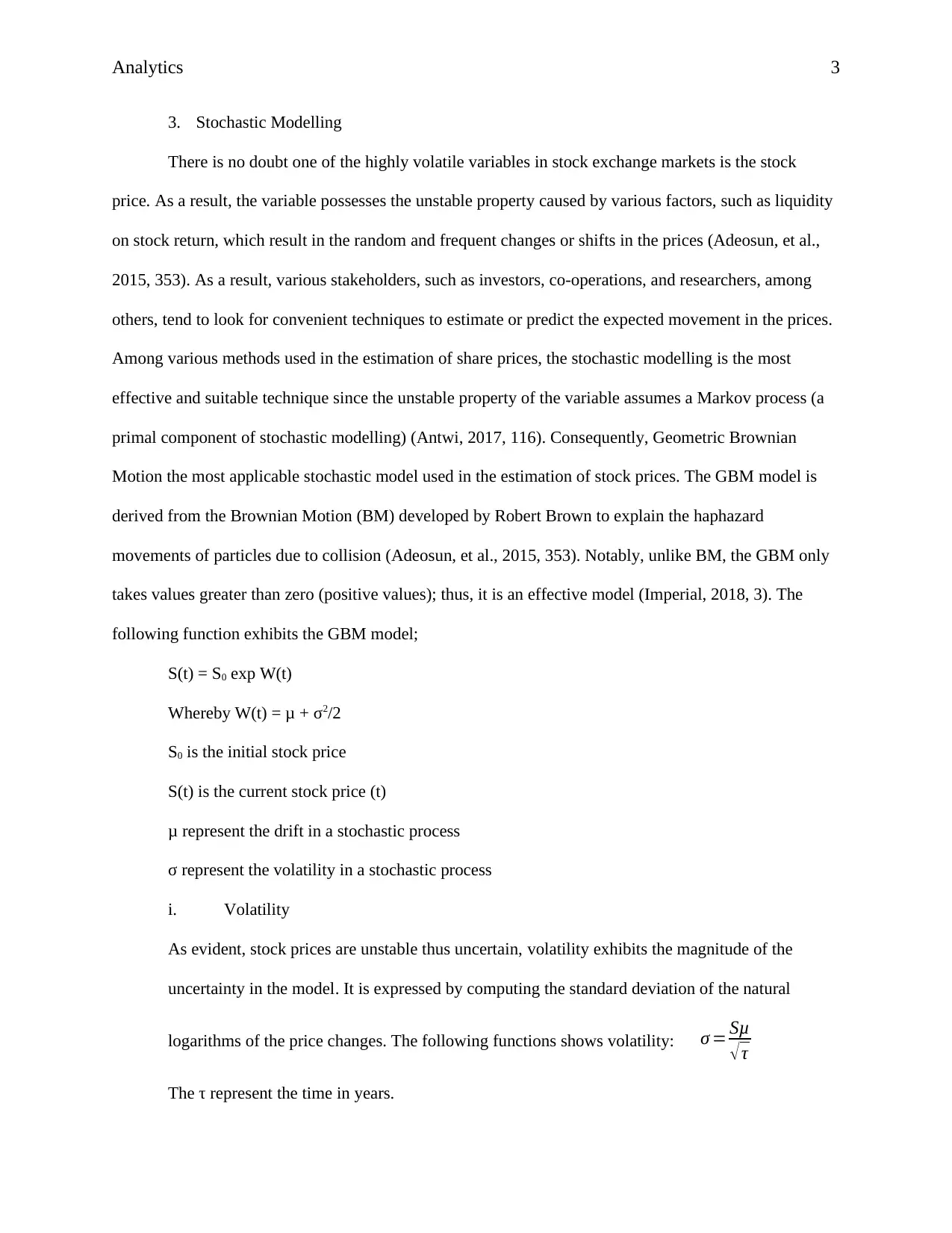
As evident, stock prices are unstable thus uncertain, volatility exhibits the magnitude of the
uncertainty in the model. It is expressed by computing the standard deviation of the natural
logarithms of the price changes. The following functions shows volatility: σ = Sμ
√ τ
The τ represent the time in years.

Analytics 4
Notably, to estimate the daily volatility the SD of a given period is computed whereas the annual
volatility is computed by multiplying the SD by the root of 252 (trading days in a year) (Adeosun,
et al., 2015, 356).
Daily Volatility = σ = Sμ
√τ
Annual volatility = σ = Sμ
√τ * √252
ii. Drift
As evident, stock prices tend to experience frequent random movements, thus drift exhibits the
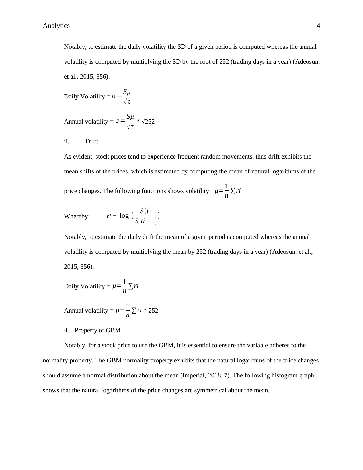
mean shifts of the prices, which is estimated by computing the mean of natural logarithms of the
price changes. The following functions shows volatility: μ= 1
n ∑ri
Whereby; ri = log ( S ( t )
S ( ti−1 ) ).
Notably, to estimate the daily drift the mean of a given period is computed whereas the annual
volatility is computed by multiplying the mean by 252 (trading days in a year) (Adeosun, et al.,
2015, 356).
Daily Volatility = μ= 1
n ∑ri
Annual volatility = μ= 1
n ∑ri * 252
4. Property of GBM
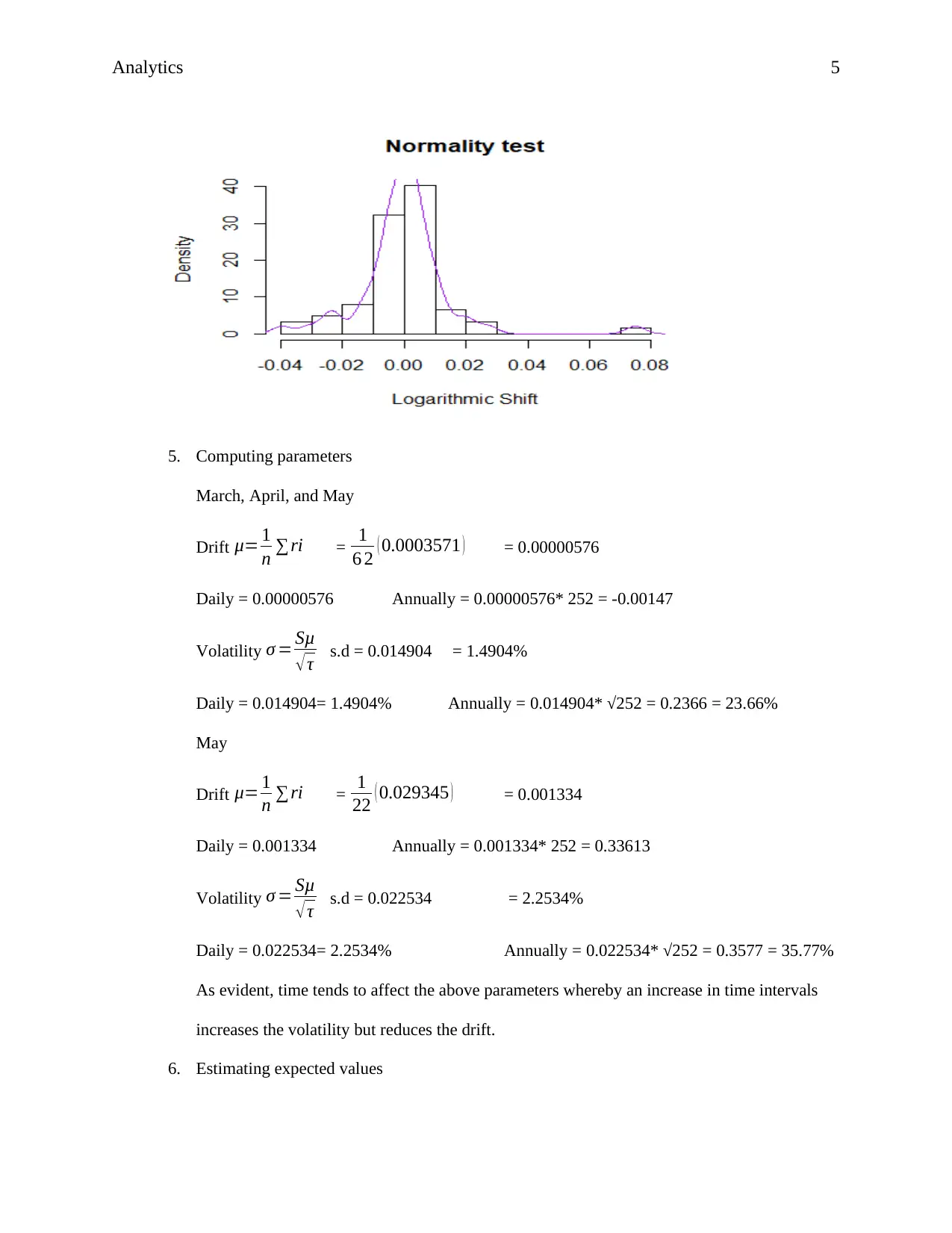
Notably, for a stock price to use the GBM, it is essential to ensure the variable adheres to the
normality property. The GBM normality property exhibits that the natural logarithms of the price changes
should assume a normal distribution about the mean (Imperial, 2018, 7). The following histogram graph
shows that the natural logarithms of the price changes are symmetrical about the mean.

Analytics 5
5. Computing parameters
March, April, and May
Drift μ= 1
n ∑ri = 1
6 2 ( 0.0003571 ) = 0.00000576
Daily = 0.00000576 Annually = 0.00000576* 252 = -0.00147
Volatility σ = Sμ
√τ s.d = 0.014904 = 1.4904%
Daily = 0.014904= 1.4904% Annually = 0.014904* √252 = 0.2366 = 23.66%
May
Drift μ= 1
n ∑ri = 1
22 ( 0.029345 ) = 0.001334
Daily = 0.001334 Annually = 0.001334* 252 = 0.33613
Volatility σ = Sμ
√τ s.d = 0.022534 = 2.2534%
Daily = 0.022534= 2.2534% Annually = 0.022534* √252 = 0.3577 = 35.77%
As evident, time tends to affect the above parameters whereby an increase in time intervals
increases the volatility but reduces the drift.
6. Estimating expected values

Analytics 6
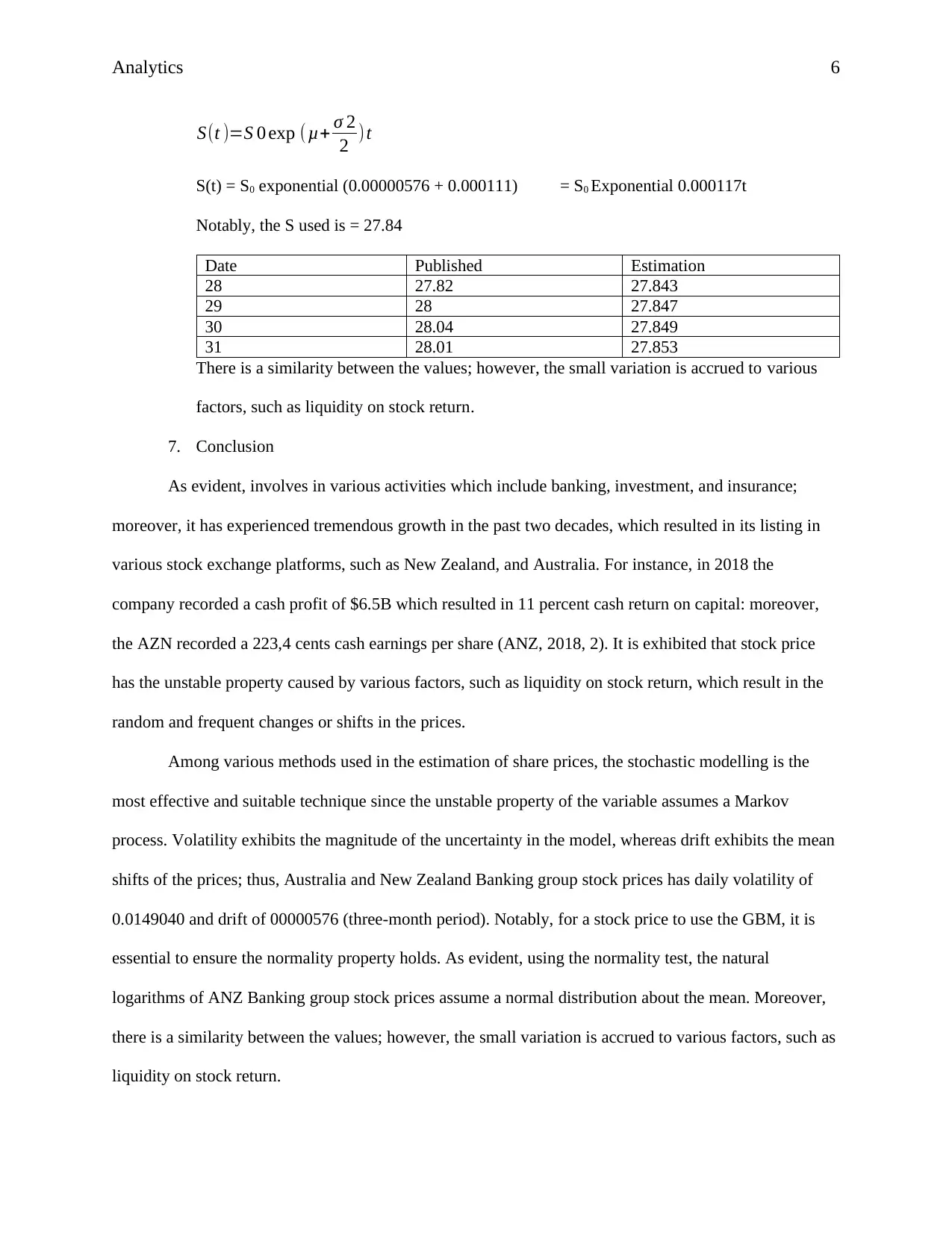
S(t )=S 0 exp (μ+ σ 2
2 )t
S(t) = S0 exponential (0.00000576 + 0.000111) = S0 Exponential 0.000117t
Notably, the S used is = 27.84
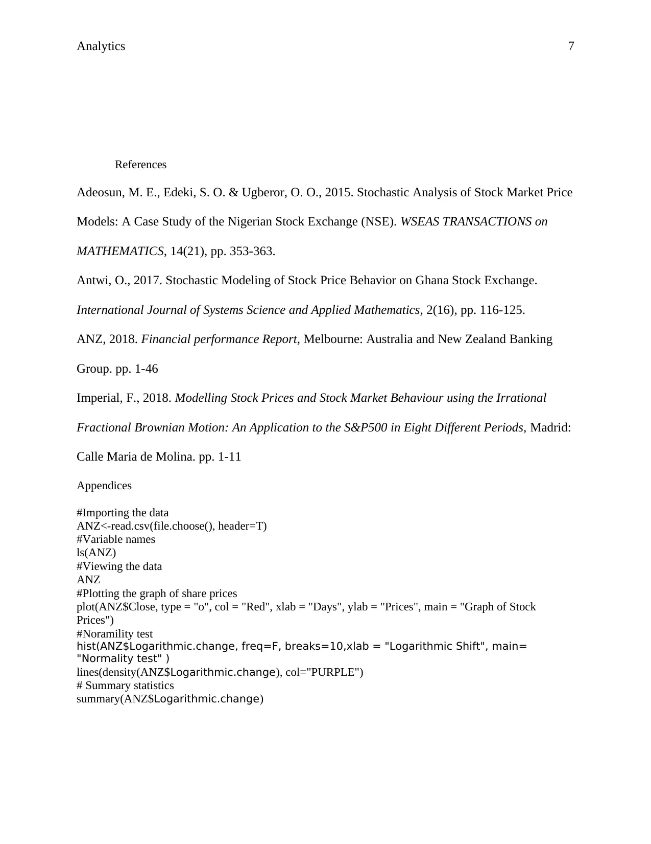
Date Published Estimation
28 27.82 27.843
29 28 27.847
30 28.04 27.849
31 28.01 27.853
There is a similarity between the values; however, the small variation is accrued to various
factors, such as liquidity on stock return.
7. Conclusion
As evident, involves in various activities which include banking, investment, and insurance;
moreover, it has experienced tremendous growth in the past two decades, which resulted in its listing in
various stock exchange platforms, such as New Zealand, and Australia. For instance, in 2018 the
company recorded a cash profit of $6.5B which resulted in 11 percent cash return on capital: moreover,
the AZN recorded a 223,4 cents cash earnings per share (ANZ, 2018, 2). It is exhibited that stock price
has the unstable property caused by various factors, such as liquidity on stock return, which result in the
random and frequent changes or shifts in the prices.
Among various methods used in the estimation of share prices, the stochastic modelling is the
most effective and suitable technique since the unstable property of the variable assumes a Markov
process. Volatility exhibits the magnitude of the uncertainty in the model, whereas drift exhibits the mean
shifts of the prices; thus, Australia and New Zealand Banking group stock prices has daily volatility of
0.0149040 and drift of 00000576 (three-month period). Notably, for a stock price to use the GBM, it is
essential to ensure the normality property holds. As evident, using the normality test, the natural
logarithms of ANZ Banking group stock prices assume a normal distribution about the mean. Moreover,
there is a similarity between the values; however, the small variation is accrued to various factors, such as
liquidity on stock return.

Analytics 7
References
Adeosun, M. E., Edeki, S. O. & Ugberor, O. O., 2015. Stochastic Analysis of Stock Market Price
Models: A Case Study of the Nigerian Stock Exchange (NSE). WSEAS TRANSACTIONS on
MATHEMATICS, 14(21), pp. 353-363.
Antwi, O., 2017. Stochastic Modeling of Stock Price Behavior on Ghana Stock Exchange.
International Journal of Systems Science and Applied Mathematics, 2(16), pp. 116-125.
ANZ, 2018. Financial performance Report, Melbourne: Australia and New Zealand Banking
Group. pp. 1-46
Imperial, F., 2018. Modelling Stock Prices and Stock Market Behaviour using the Irrational
Fractional Brownian Motion: An Application to the S&P500 in Eight Different Periods, Madrid:
Calle Maria de Molina. pp. 1-11
Appendices
#Importing the data
ANZ<-read.csv(file.choose(), header=T)
#Variable names
ls(ANZ)
#Viewing the data
ANZ
#Plotting the graph of share prices
plot(ANZ$Close, type = "o", col = "Red", xlab = "Days", ylab = "Prices", main = "Graph of Stock
Prices")
#Noramility test
hist(ANZ$Logarithmic.change, freq=F, breaks=10,xlab = "Logarithmic Shift", main=
"Normality test" )
lines(density(ANZ$Logarithmic.change), col="PURPLE")
# Summary statistics
summary(ANZ$Logarithmic.change)