SIT720: Machine Learning Project - Classification Techniques

This machine learning project explores several classification techniques, including K-Nearest Neighbor (KNN), Multiclass Logistic Regression with Elastic Net, Support Vector Machine (SVM) with RBF kernel, and Random Forest. The project begins with data understanding, examining the dataset's characteristics and features. Subsequently, each classification technique is implemented and evaluated using Python, with a focus on model performance, cross-validation, and the F1 score. The KNN model utilizes a 10-fold cross-validation, with the optimal k value determined through grid search. The logistic regression model employs elastic net regularization, and the SVM model utilizes the RBF kernel. The Random Forest model is implemented and evaluated. The project concludes with a comparison of the different models, identifying the SVM model as the most promising, and providing insights into the strengths and weaknesses of each approach.

Machine Learning
Contents
Introduction.................................................................................................................................................1
Task A: Understanding of the data..............................................................................................................1
Task B: K-Nearest Neighbor Classification...................................................................................................2
Task C: Multiclass Logistic Regression with Elastic Net................................................................................6
Task D: Support Vector Machine ( RBF Kernal)............................................................................................9
Task E: Random Forest..............................................................................................................................11
Task F: Comparison of the different models..............................................................................................12
References:................................................................................................................................................14
List of Figures
Figure 1 Cross validation for the KNN model...............................................................................................6
Figure 2 Cross validation plot for the logistic regression.............................................................................9
Figure 3 Cross validation for the SVM model.............................................................................................11
Figure 4 Cross validation plot for the random forest.................................................................................13
List of Tables
Table 1 overview of the data.......................................................................................................................3
Table 2 calculating the f1 score for KNN model...........................................................................................4
Table 3 Results of Grid Search for the logistic regression............................................................................8
Table 4 Results from the GridSearch for random forest............................................................................12

Introduction
Machine learning and data analytics has become an important part of every industry ranging
from the FMCG companies to the health care and the logistics industries. Availability of
different types of data (both structured and the unstructured data) and the analytical and
statistical techniques has helped various industries to make better business decisions(Acharjya &
P 2016; Xie et al. 2018). From predicting the weather to predicting the customer purchasing
behavior data analytics has become important part of every business. So, in the project is also
aimed to implement some of the machine learning techniques and interpret the findings. This
project will focus majorly on the classification techniques. Some of the classification techniques
included in the current project are the random forest, support vector machine, KNN and the
logistic regression. All the techniques have been tested on the same data set so that the
comparison can be made. The comparison of the models and identification of the best model has
been presented in the last part of the project.
Task A: Understanding of the data
The first part is focused on the understanding the given data set from various perspective. For
analysis, whether it is a big or small, the understanding of the data is very important. Until and
unless the data is understood properly, the appropriate analysis cannot be performed. In other
words, to find useful information from the given data, understanding of the given data is very
important(Ziafat & Shakeri 2014). In this section, the understanding of the data has been done on
the basis of the aim and the number of the data points in the data set.
As the data and the given guidelines suggests, the main objective of the current data analysis
project is to use the different analytical and statistical techniques and profile the
customers/individual’s behavior. In other words classifying the individuals in different groups
based on their behavior.
Data from both the train and test data set shows that there are different kinds of activities
included in the research. These are the daily activities of the human beings or more specifically
the physical activities. Some of them are walking, lying down, climbing the stairs, sitting etc.
In terms of the data, the total number of rows are 7352, which means there are 7352 instances,
whereas the data shows that the number of columns are 561 which are also the number of
features. Data also shows that the data was collected among 30 different individuals.
While talking about the results, among the different classification techniques used in the study,
the results from the SVM method shows the most promising results with 96 % accuracy.

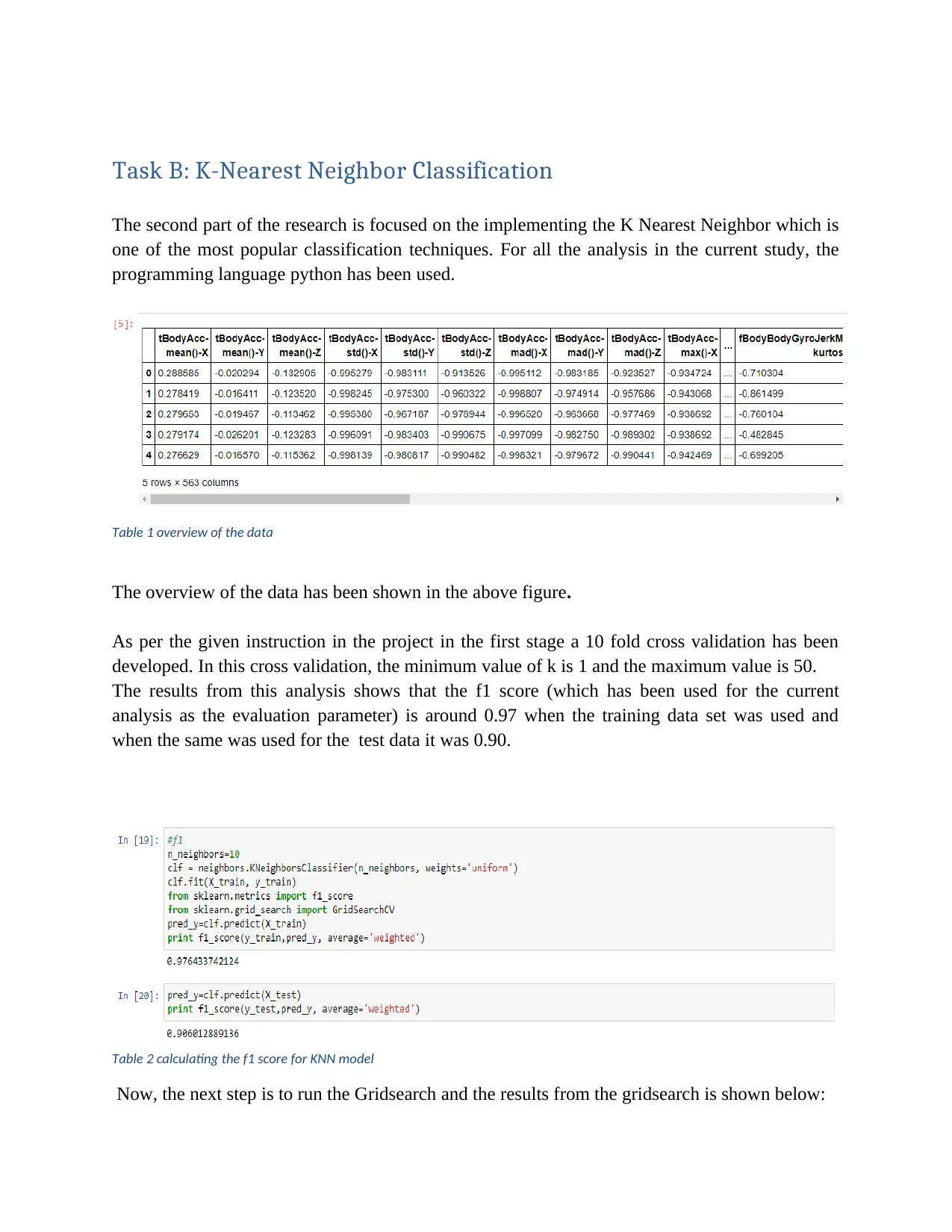
Task B: K-Nearest Neighbor Classification
The second part of the research is focused on the implementing the K Nearest Neighbor which is
one of the most popular classification techniques. For all the analysis in the current study, the
programming language python has been used.
Table 1 overview of the data
The overview of the data has been shown in the above figure.
As per the given instruction in the project in the first stage a 10 fold cross validation has been
developed. In this cross validation, the minimum value of k is 1 and the maximum value is 50.
The results from this analysis shows that the f1 score (which has been used for the current
analysis as the evaluation parameter) is around 0.97 when the training data set was used and
when the same was used for the test data it was 0.90.
Table 2 calculating the f1 score for KNN model
Now, the next step is to run the Gridsearch and the results from the gridsearch is shown below:

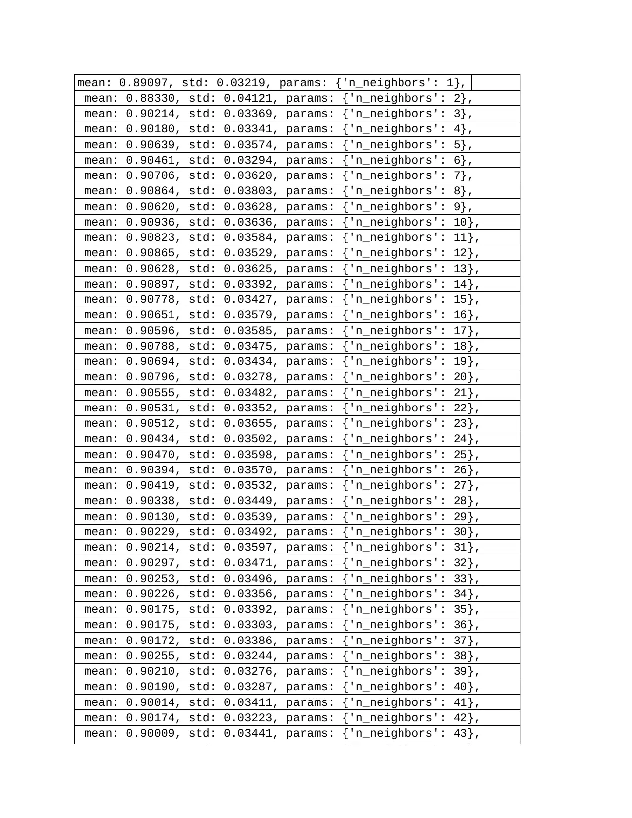
mean: 0.89097, std: 0.03219, params: {'n_neighbors': 1},
mean: 0.88330, std: 0.04121, params: {'n_neighbors': 2},
mean: 0.90214, std: 0.03369, params: {'n_neighbors': 3},
mean: 0.90180, std: 0.03341, params: {'n_neighbors': 4},
mean: 0.90639, std: 0.03574, params: {'n_neighbors': 5},
mean: 0.90461, std: 0.03294, params: {'n_neighbors': 6},
mean: 0.90706, std: 0.03620, params: {'n_neighbors': 7},
mean: 0.90864, std: 0.03803, params: {'n_neighbors': 8},
mean: 0.90620, std: 0.03628, params: {'n_neighbors': 9},
mean: 0.90936, std: 0.03636, params: {'n_neighbors': 10},
mean: 0.90823, std: 0.03584, params: {'n_neighbors': 11},
mean: 0.90865, std: 0.03529, params: {'n_neighbors': 12},
mean: 0.90628, std: 0.03625, params: {'n_neighbors': 13},
mean: 0.90897, std: 0.03392, params: {'n_neighbors': 14},
mean: 0.90778, std: 0.03427, params: {'n_neighbors': 15},
mean: 0.90651, std: 0.03579, params: {'n_neighbors': 16},
mean: 0.90596, std: 0.03585, params: {'n_neighbors': 17},
mean: 0.90788, std: 0.03475, params: {'n_neighbors': 18},
mean: 0.90694, std: 0.03434, params: {'n_neighbors': 19},
mean: 0.90796, std: 0.03278, params: {'n_neighbors': 20},
mean: 0.90555, std: 0.03482, params: {'n_neighbors': 21},
mean: 0.90531, std: 0.03352, params: {'n_neighbors': 22},
mean: 0.90512, std: 0.03655, params: {'n_neighbors': 23},
mean: 0.90434, std: 0.03502, params: {'n_neighbors': 24},
mean: 0.90470, std: 0.03598, params: {'n_neighbors': 25},
mean: 0.90394, std: 0.03570, params: {'n_neighbors': 26},
mean: 0.90419, std: 0.03532, params: {'n_neighbors': 27},
mean: 0.90338, std: 0.03449, params: {'n_neighbors': 28},
mean: 0.90130, std: 0.03539, params: {'n_neighbors': 29},
mean: 0.90229, std: 0.03492, params: {'n_neighbors': 30},
mean: 0.90214, std: 0.03597, params: {'n_neighbors': 31},
mean: 0.90297, std: 0.03471, params: {'n_neighbors': 32},
mean: 0.90253, std: 0.03496, params: {'n_neighbors': 33},
mean: 0.90226, std: 0.03356, params: {'n_neighbors': 34},
mean: 0.90175, std: 0.03392, params: {'n_neighbors': 35},
mean: 0.90175, std: 0.03303, params: {'n_neighbors': 36},
mean: 0.90172, std: 0.03386, params: {'n_neighbors': 37},
mean: 0.90255, std: 0.03244, params: {'n_neighbors': 38},
mean: 0.90210, std: 0.03276, params: {'n_neighbors': 39},
mean: 0.90190, std: 0.03287, params: {'n_neighbors': 40},
mean: 0.90014, std: 0.03411, params: {'n_neighbors': 41},
mean: 0.90174, std: 0.03223, params: {'n_neighbors': 42},
mean: 0.90009, std: 0.03441, params: {'n_neighbors': 43},
mean: 0.90070, std: 0.03303, params: {'n_neighbors': 44},
mean: 0.90039, std: 0.03331, params: {'n_neighbors': 45},
mean: 0.90047, std: 0.03249, params: {'n_neighbors': 46},
mean: 0.89809, std: 0.03393, params: {'n_neighbors': 47},
mean: 0.89939, std: 0.03262, params: {'n_neighbors': 48},

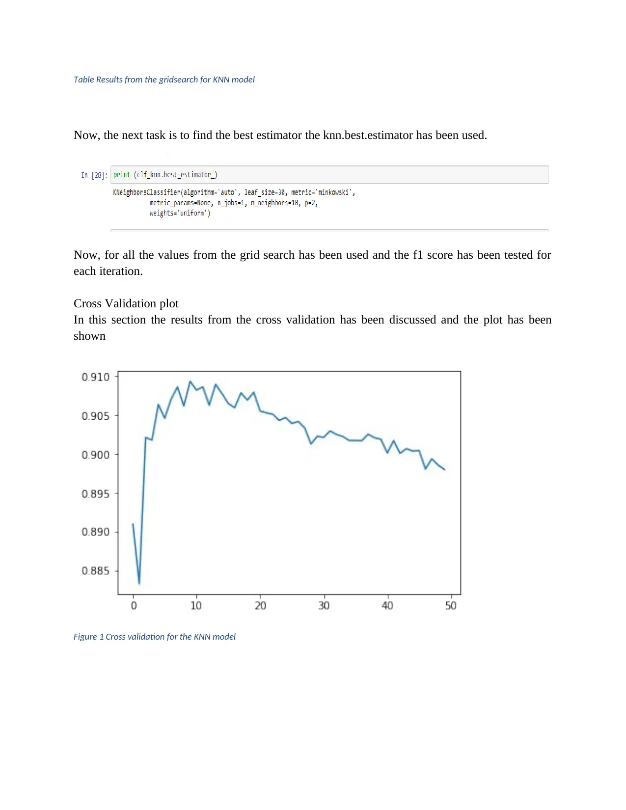
Table Results from the gridsearch for KNN model
Now, the next task is to find the best estimator the knn.best.estimator has been used.
Now, for all the values from the grid search has been used and the f1 score has been tested for
each iteration.
Cross Validation plot
In this section the results from the cross validation has been discussed and the plot has been
shown
Figure 1 Cross validation for the KNN model

.
On the basis of the results from the cross validation, the f1 score continue to increase till k = 10.
In fact f1 is highest when k = 10. After that the f1 value declines. So, on the basis of this results
the accuracy score and the confusion matrix has been constructed.
0.906012889136
0.906684764167
[[534 2 1 0 0 0]
[ 0 409 78 0 0 4]
[ 0 47 485 0 0 0]
[ 0 0 0 486 10 0]
[ 0 0 0 51 331 38]
[ 0 0 0 36 8 427]]
As the results show the f1 value is 0.90 and also the value of accuracy is 0.90. So, it can be
concluded that our model is 90 % accurate.
Task C: Multiclass Logistic Regression with Elastic Net
Another model used in the current project is the Multiple logistics model and the results from the
model are discussed in the current section (Armstrong 2012; Cerrito 2010; George, Seals &
Aban 2014).
The results from the gridsearch for logistic regresion is shown below:

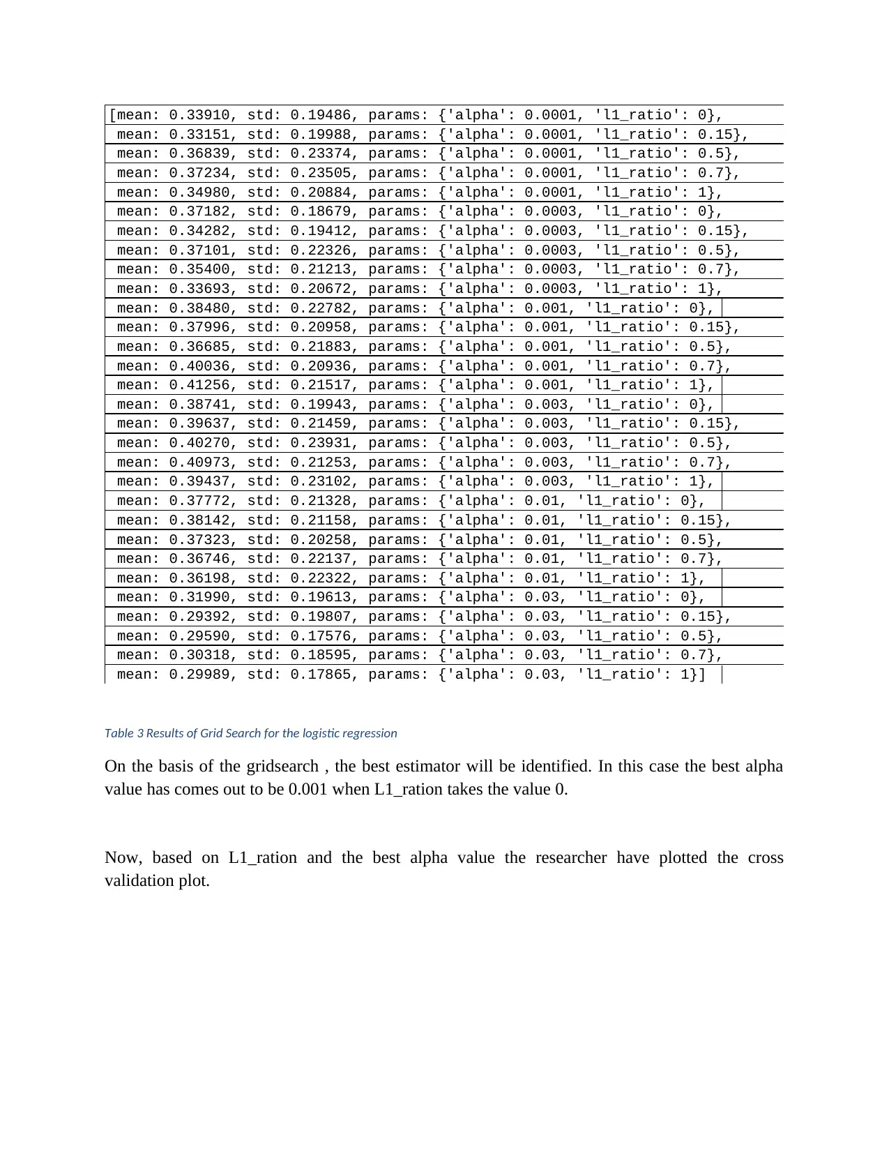
[mean: 0.33910, std: 0.19486, params: {'alpha': 0.0001, 'l1_ratio': 0},
mean: 0.33151, std: 0.19988, params: {'alpha': 0.0001, 'l1_ratio': 0.15},
mean: 0.36839, std: 0.23374, params: {'alpha': 0.0001, 'l1_ratio': 0.5},
mean: 0.37234, std: 0.23505, params: {'alpha': 0.0001, 'l1_ratio': 0.7},
mean: 0.34980, std: 0.20884, params: {'alpha': 0.0001, 'l1_ratio': 1},
mean: 0.37182, std: 0.18679, params: {'alpha': 0.0003, 'l1_ratio': 0},
mean: 0.34282, std: 0.19412, params: {'alpha': 0.0003, 'l1_ratio': 0.15},
mean: 0.37101, std: 0.22326, params: {'alpha': 0.0003, 'l1_ratio': 0.5},
mean: 0.35400, std: 0.21213, params: {'alpha': 0.0003, 'l1_ratio': 0.7},
mean: 0.33693, std: 0.20672, params: {'alpha': 0.0003, 'l1_ratio': 1},
mean: 0.38480, std: 0.22782, params: {'alpha': 0.001, 'l1_ratio': 0},
mean: 0.37996, std: 0.20958, params: {'alpha': 0.001, 'l1_ratio': 0.15},
mean: 0.36685, std: 0.21883, params: {'alpha': 0.001, 'l1_ratio': 0.5},
mean: 0.40036, std: 0.20936, params: {'alpha': 0.001, 'l1_ratio': 0.7},
mean: 0.41256, std: 0.21517, params: {'alpha': 0.001, 'l1_ratio': 1},
mean: 0.38741, std: 0.19943, params: {'alpha': 0.003, 'l1_ratio': 0},
mean: 0.39637, std: 0.21459, params: {'alpha': 0.003, 'l1_ratio': 0.15},
mean: 0.40270, std: 0.23931, params: {'alpha': 0.003, 'l1_ratio': 0.5},
mean: 0.40973, std: 0.21253, params: {'alpha': 0.003, 'l1_ratio': 0.7},
mean: 0.39437, std: 0.23102, params: {'alpha': 0.003, 'l1_ratio': 1},
mean: 0.37772, std: 0.21328, params: {'alpha': 0.01, 'l1_ratio': 0},
mean: 0.38142, std: 0.21158, params: {'alpha': 0.01, 'l1_ratio': 0.15},
mean: 0.37323, std: 0.20258, params: {'alpha': 0.01, 'l1_ratio': 0.5},
mean: 0.36746, std: 0.22137, params: {'alpha': 0.01, 'l1_ratio': 0.7},
mean: 0.36198, std: 0.22322, params: {'alpha': 0.01, 'l1_ratio': 1},
mean: 0.31990, std: 0.19613, params: {'alpha': 0.03, 'l1_ratio': 0},
mean: 0.29392, std: 0.19807, params: {'alpha': 0.03, 'l1_ratio': 0.15},
mean: 0.29590, std: 0.17576, params: {'alpha': 0.03, 'l1_ratio': 0.5},
mean: 0.30318, std: 0.18595, params: {'alpha': 0.03, 'l1_ratio': 0.7},
mean: 0.29989, std: 0.17865, params: {'alpha': 0.03, 'l1_ratio': 1}]
Table 3 Results of Grid Search for the logistic regression
On the basis of the gridsearch , the best estimator will be identified. In this case the best alpha
value has comes out to be 0.001 when L1_ration takes the value 0.
Now, based on L1_ration and the best alpha value the researcher have plotted the cross
validation plot.

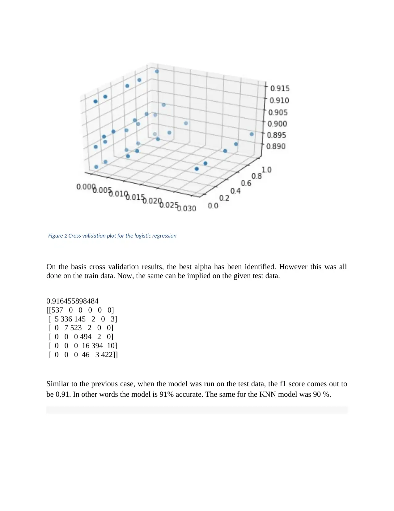
Figure 2 Cross validation plot for the logistic regression
On the basis cross validation results, the best alpha has been identified. However this was all
done on the train data. Now, the same can be implied on the given test data.
0.916455898484
[[537 0 0 0 0 0]
[ 5 336 145 2 0 3]
[ 0 7 523 2 0 0]
[ 0 0 0 494 2 0]
[ 0 0 0 16 394 10]
[ 0 0 0 46 3 422]]
Similar to the previous case, when the model was run on the test data, the f1 score comes out to
be 0.91. In other words the model is 91% accurate. The same for the KNN model was 90 %.

Task D: Support Vector Machine ( RBF Kernal)
In this fourth section another popular classification technique has been discussed and this
technique is SVM or Support Vector Machine. In this the RBF kernel will be used (Bhavsar &
Panchal 2012).
In this case the SVM has been optimized on the basis of the following two parameters:
The first one is “C” which is the penalty meter of the error term. Whereas the second is the
“Gamma” which is described as the kernel coefficient for the functional form.
In this case also the grisearch has been used for the purpose of tuning the given hyper
parameters and the SVM best estimator has been identified. .
Identification of classification of SVM best estimator:
The value of C and Gamma are as follows:
{'gamma': [ 1e-3, 1e-4],
'C':[1, 10, 100, 1000]}
On the basis of the above results, the optimal values are:
C = 1000
gamma value= 0.001
Now, the next step is to plot the cross validation plot on the basis of the given “C” and
“Gamma”.

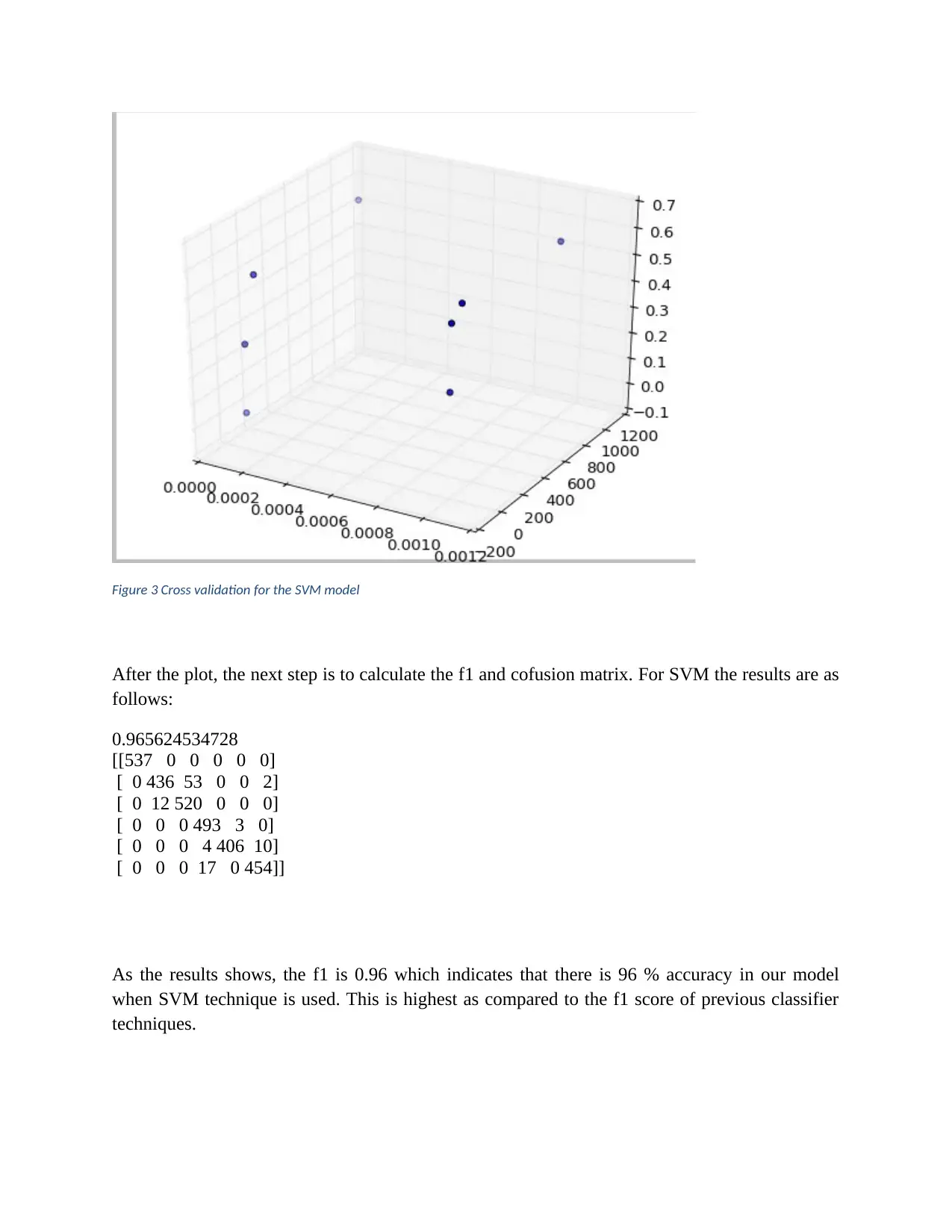
Figure 3 Cross validation for the SVM model
After the plot, the next step is to calculate the f1 and cofusion matrix. For SVM the results are as
follows:
0.965624534728
[[537 0 0 0 0 0]
[ 0 436 53 0 0 2]
[ 0 12 520 0 0 0]
[ 0 0 0 493 3 0]
[ 0 0 0 4 406 10]
[ 0 0 0 17 0 454]]
As the results shows, the f1 is 0.96 which indicates that there is 96 % accuracy in our model
when SVM technique is used. This is highest as compared to the f1 score of previous classifier
techniques.

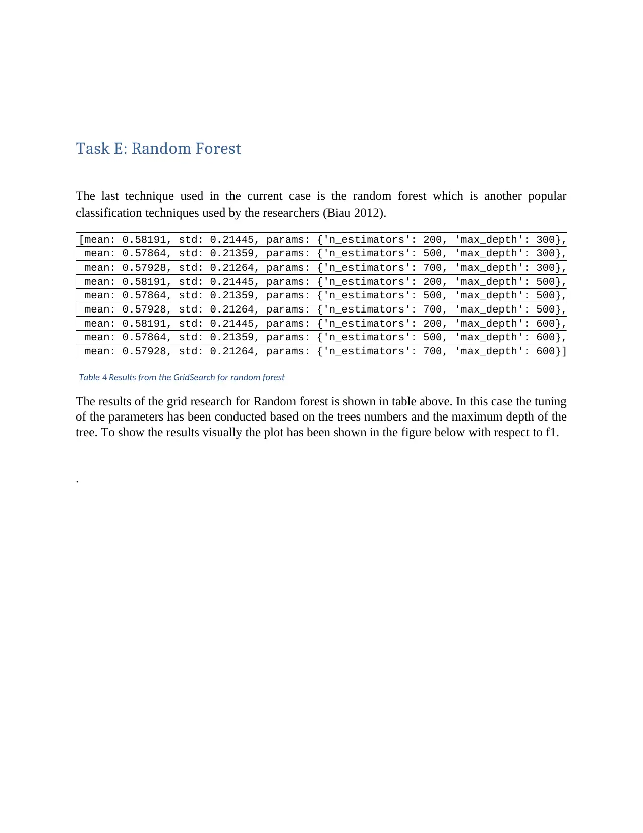
Task E: Random Forest
The last technique used in the current case is the random forest which is another popular
classification techniques used by the researchers (Biau 2012).
[mean: 0.58191, std: 0.21445, params: {'n_estimators': 200, 'max_depth': 300},
mean: 0.57864, std: 0.21359, params: {'n_estimators': 500, 'max_depth': 300},
mean: 0.57928, std: 0.21264, params: {'n_estimators': 700, 'max_depth': 300},
mean: 0.58191, std: 0.21445, params: {'n_estimators': 200, 'max_depth': 500},
mean: 0.57864, std: 0.21359, params: {'n_estimators': 500, 'max_depth': 500},
mean: 0.57928, std: 0.21264, params: {'n_estimators': 700, 'max_depth': 500},
mean: 0.58191, std: 0.21445, params: {'n_estimators': 200, 'max_depth': 600},
mean: 0.57864, std: 0.21359, params: {'n_estimators': 500, 'max_depth': 600},
mean: 0.57928, std: 0.21264, params: {'n_estimators': 700, 'max_depth': 600}]
Table 4 Results from the GridSearch for random forest
The results of the grid research for Random forest is shown in table above. In this case the tuning
of the parameters has been conducted based on the trees numbers and the maximum depth of the
tree. To show the results visually the plot has been shown in the figure below with respect to f1.
.