FIN200 Assignment: Analyzing SML, CML, Minimum Variance, and CAPM

This report provides a comprehensive analysis of key concepts in corporate financial accounting, including the Security Market Line (SML), Capital Market Line (CML), minimum variance portfolios, and the Capital Asset Pricing Model (CAPM). It elucidates the differences between SML and CML, highlighting their graphical representations and risk measurement methodologies. The report also explores the importance of minimum variance portfolios in mitigating risk through diversification and hedging strategies. Furthermore, it justifies the relevance of the CAPM equation in calculating the required rate of return by considering both the time value of money and risk premium, offering insights into investment decision-making processes.

CORPORATE FINANCIAL ACCOUNTING

INTRODUCTION
In the world of technology and advancements, the share market is one of the most dynamic fields
affected by the forces of demand and supply (Adelaja, 2015).
For the fruitful investment decisions to be made in the market, it is important that one should
have a clear idea about the forces of market. There is a much known concept called portfolio
analysis. Analysis of stocks on an individual basis and analysis of the entire portfolio is
important for the investor's decision making as investors expect returns and returns are possible
only when the market is rising or the economy is growing and a complete idea is available to the
investors. However, the analysis of the market is a broad concept that makes use of various other
concepts such as CAPM, CML, CAL and SML discussed in details below.

SECURITY MARKET LINE
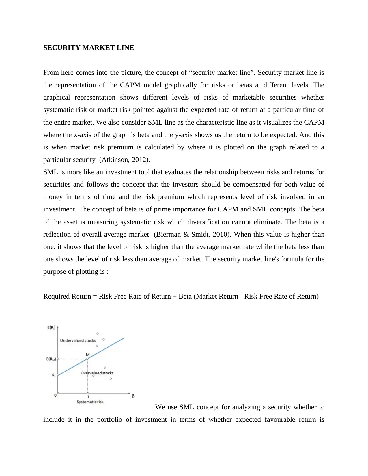
From here comes into the picture, the concept of “security market line”. Security market line is
the representation of the CAPM model graphically for risks or betas at different levels. The
graphical representation shows different levels of risks of marketable securities whether
systematic risk or market risk pointed against the expected rate of return at a particular time of
the entire market. We also consider SML line as the characteristic line as it visualizes the CAPM
where the x-axis of the graph is beta and the y-axis shows us the return to be expected. And this
is when market risk premium is calculated by where it is plotted on the graph related to a
particular security (Atkinson, 2012).
SML is more like an investment tool that evaluates the relationship between risks and returns for
securities and follows the concept that the investors should be compensated for both value of
money in terms of time and the risk premium which represents level of risk involved in an
investment. The concept of beta is of prime importance for CAPM and SML concepts. The beta
of the asset is measuring systematic risk which diversification cannot eliminate. The beta is a
reflection of overall average market (Bierman & Smidt, 2010). When this value is higher than
one, it shows that the level of risk is higher than the average market rate while the beta less than
one shows the level of risk less than average of market. The security market line's formula for the
purpose of plotting is :
Required Return = Risk Free Rate of Return + Beta (Market Return - Risk Free Rate of Return)
We use SML concept for analyzing a security whether to
include it in the portfolio of investment in terms of whether expected favourable return is

received or not against its risk level. When the security is plotted above the SML, the security is
considered to be undervalued because that means that the security offers a return which is way
greater than its risk (Dayananda, Irons, Harrison, Herbohn, & Rowland, 2008). On the other
hand, in case of vice - versa, the stock is considered as overvalued in terms of price because in
that case, the expected return doesn't exceed the risks involved. The frequent use of SML is in
comparing the two securities of similar nature that offers almost same return in order ro estimate
that which security involves the minimum level of risk involved in relation to expected return. In
a similar way, two stocks are compared with equal risk that which security offers highest
expected return.
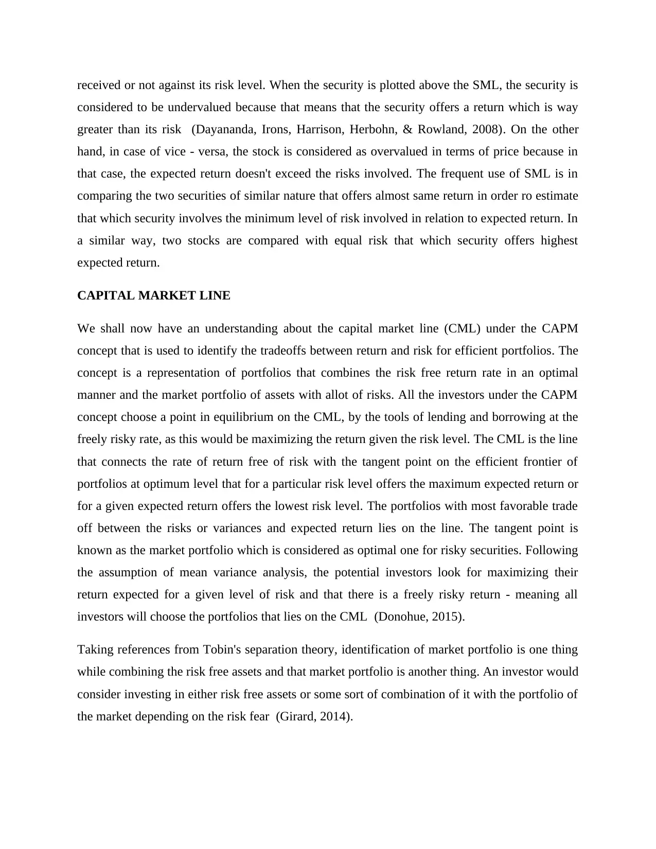
CAPITAL MARKET LINE
We shall now have an understanding about the capital market line (CML) under the CAPM
concept that is used to identify the tradeoffs between return and risk for efficient portfolios. The
concept is a representation of portfolios that combines the risk free return rate in an optimal
manner and the market portfolio of assets with allot of risks. All the investors under the CAPM
concept choose a point in equilibrium on the CML, by the tools of lending and borrowing at the
freely risky rate, as this would be maximizing the return given the risk level. The CML is the line
that connects the rate of return free of risk with the tangent point on the efficient frontier of
portfolios at optimum level that for a particular risk level offers the maximum expected return or
for a given expected return offers the lowest risk level. The portfolios with most favorable trade
off between the risks or variances and expected return lies on the line. The tangent point is
known as the market portfolio which is considered as optimal one for risky securities. Following
the assumption of mean variance analysis, the potential investors look for maximizing their
return expected for a given level of risk and that there is a freely risky return - meaning all
investors will choose the portfolios that lies on the CML (Donohue, 2015).
Taking references from Tobin's separation theory, identification of market portfolio is one thing
while combining the risk free assets and that market portfolio is another thing. An investor would
consider investing in either risk free assets or some sort of combination of it with the portfolio of
the market depending on the risk fear (Girard, 2014).

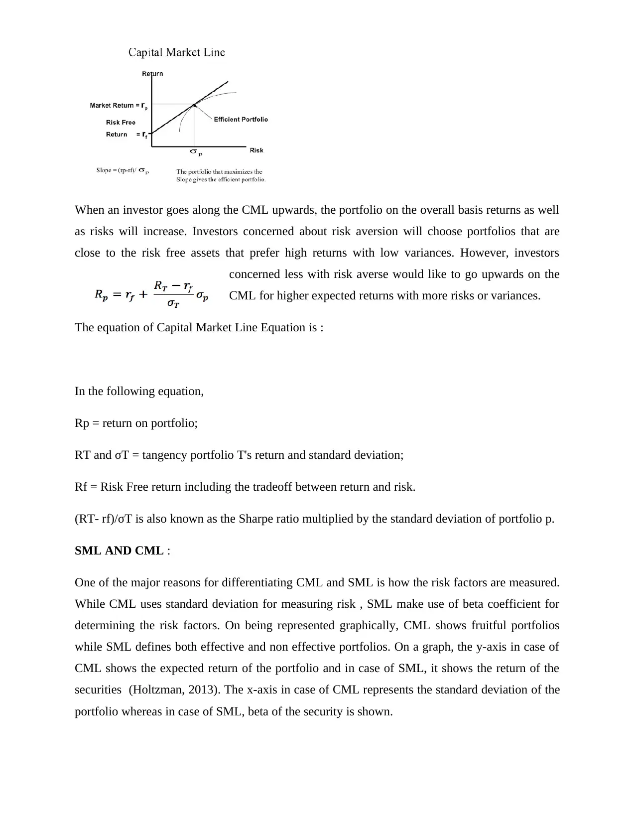
When an investor goes along the CML upwards, the portfolio on the overall basis returns as well
as risks will increase. Investors concerned about risk aversion will choose portfolios that are
close to the risk free assets that prefer high returns with low variances. However, investors
concerned less with risk averse would like to go upwards on the
CML for higher expected returns with more risks or variances.
The equation of Capital Market Line Equation is :
In the following equation,
Rp = return on portfolio;
RT and σT = tangency portfolio T's return and standard deviation;
Rf = Risk Free return including the tradeoff between return and risk.
(RT- rf)/σT is also known as the Sharpe ratio multiplied by the standard deviation of portfolio p.
SML AND CML :
One of the major reasons for differentiating CML and SML is how the risk factors are measured.
While CML uses standard deviation for measuring risk , SML make use of beta coefficient for
determining the risk factors. On being represented graphically, CML shows fruitful portfolios
while SML defines both effective and non effective portfolios. On a graph, the y-axis in case of
CML shows the expected return of the portfolio and in case of SML, it shows the return of the
securities (Holtzman, 2013). The x-axis in case of CML represents the standard deviation of the
portfolio whereas in case of SML, beta of the security is shown.

CML shows the risk free assets and market portfolio while SML determines the other factors of
security. SML shows the expected returns on an individual basis in case of all securities unlike
CML. While CML determines the return or risks for efficient portfolios, SML determines the
return or risks associated with individual stocks. However, SML can be a tool valued enough for
valuation of equity and comparison purposes; it shouldn't be use for isolation purposes as the
expected return rate over risk free return rate is not considered as the only reason for decision
making related to investment. That is why, capital market line is considered better when it comes
to measurement of risk factors (McLaney & Adril, 2016).

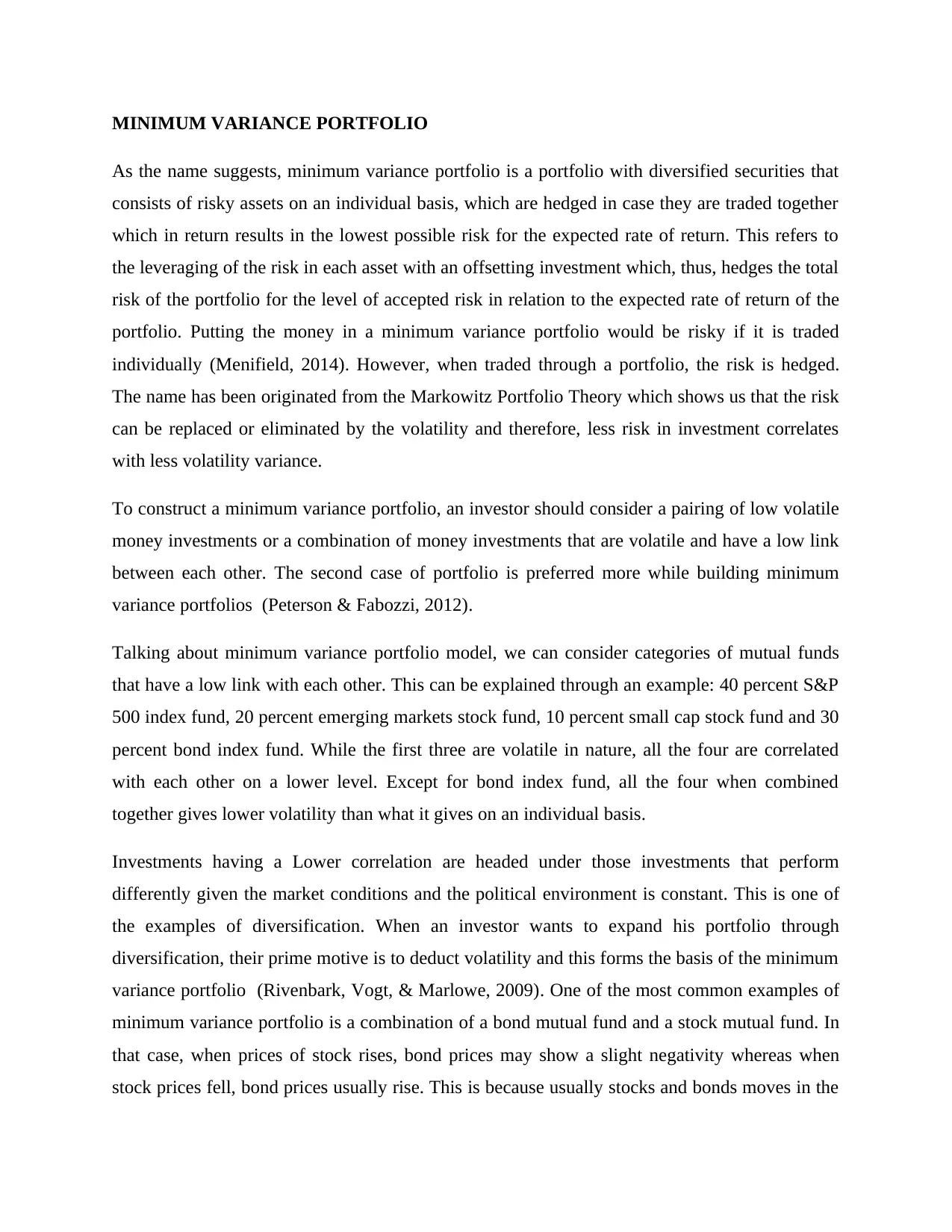
MINIMUM VARIANCE PORTFOLIO
As the name suggests, minimum variance portfolio is a portfolio with diversified securities that
consists of risky assets on an individual basis, which are hedged in case they are traded together
which in return results in the lowest possible risk for the expected rate of return. This refers to
the leveraging of the risk in each asset with an offsetting investment which, thus, hedges the total
risk of the portfolio for the level of accepted risk in relation to the expected rate of return of the
portfolio. Putting the money in a minimum variance portfolio would be risky if it is traded
individually (Menifield, 2014). However, when traded through a portfolio, the risk is hedged.
The name has been originated from the Markowitz Portfolio Theory which shows us that the risk
can be replaced or eliminated by the volatility and therefore, less risk in investment correlates
with less volatility variance.
To construct a minimum variance portfolio, an investor should consider a pairing of low volatile
money investments or a combination of money investments that are volatile and have a low link
between each other. The second case of portfolio is preferred more while building minimum
variance portfolios (Peterson & Fabozzi, 2012).
Talking about minimum variance portfolio model, we can consider categories of mutual funds
that have a low link with each other. This can be explained through an example: 40 percent S&P
500 index fund, 20 percent emerging markets stock fund, 10 percent small cap stock fund and 30
percent bond index fund. While the first three are volatile in nature, all the four are correlated
with each other on a lower level. Except for bond index fund, all the four when combined
together gives lower volatility than what it gives on an individual basis.
Investments having a Lower correlation are headed under those investments that perform
differently given the market conditions and the political environment is constant. This is one of
the examples of diversification. When an investor wants to expand his portfolio through
diversification, their prime motive is to deduct volatility and this forms the basis of the minimum
variance portfolio (Rivenbark, Vogt, & Marlowe, 2009). One of the most common examples of
minimum variance portfolio is a combination of a bond mutual fund and a stock mutual fund. In
that case, when prices of stock rises, bond prices may show a slight negativity whereas when
stock prices fell, bond prices usually rise. This is because usually stocks and bonds moves in the

same direction but they have a low correlation when it comes to performance. With minimum
variance portfolio, an investor can efficiently combine the investments together that are risky and
can still manage to achieve high returns without bearing the high risk level (Robinson, 2014).

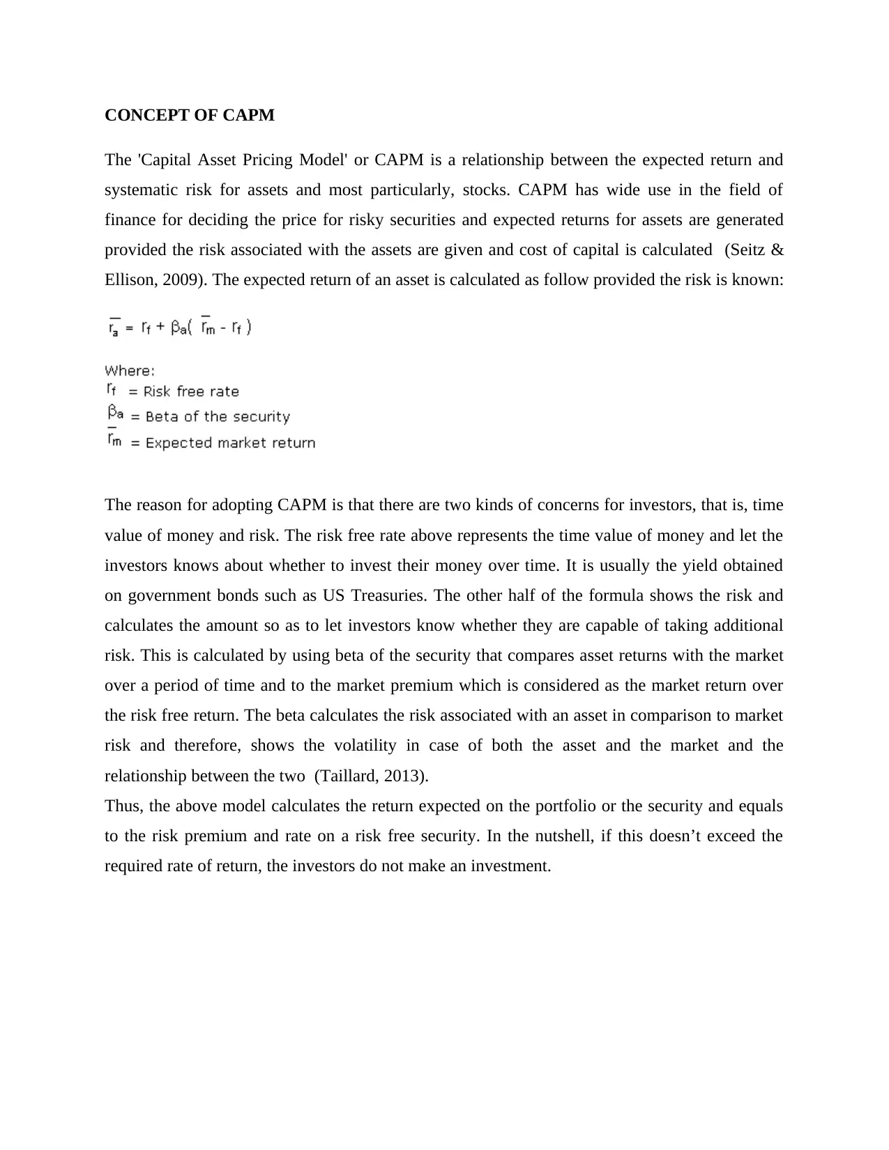
CONCEPT OF CAPM
The 'Capital Asset Pricing Model' or CAPM is a relationship between the expected return and
systematic risk for assets and most particularly, stocks. CAPM has wide use in the field of
finance for deciding the price for risky securities and expected returns for assets are generated
provided the risk associated with the assets are given and cost of capital is calculated (Seitz &
Ellison, 2009). The expected return of an asset is calculated as follow provided the risk is known:
The reason for adopting CAPM is that there are two kinds of concerns for investors, that is, time
value of money and risk. The risk free rate above represents the time value of money and let the
investors knows about whether to invest their money over time. It is usually the yield obtained
on government bonds such as US Treasuries. The other half of the formula shows the risk and
calculates the amount so as to let investors know whether they are capable of taking additional
risk. This is calculated by using beta of the security that compares asset returns with the market
over a period of time and to the market premium which is considered as the market return over
the risk free return. The beta calculates the risk associated with an asset in comparison to market
risk and therefore, shows the volatility in case of both the asset and the market and the
relationship between the two (Taillard, 2013).
Thus, the above model calculates the return expected on the portfolio or the security and equals
to the risk premium and rate on a risk free security. In the nutshell, if this doesn’t exceed the
required rate of return, the investors do not make an investment.

WHY CAPM?
"The CAPM is an important area of financial management. In fact, it has even been suggested
that finance only became ‘a fully-fledged, scientific discipline’ when William Sharpe published
his derivation of the CAPM in 1986” (Shapiro, 2007).
Being a popular concept for more than 40 years, the reasons of choosing CAPM formulas over
other formulas can be explained as below:
 A single systematic risk is considered which reflects the reality of the diversified
portfolios in which investors have an interest and an unsystematic risk is significantly
eliminated (Siciliano, 2015).
 It has derived from the relationship between systematic risk and required return through a
theoretical approach which is frequently researched about and tested on a regular basis.
 Generally, for the calculation of cost of equity, the CAPM approach is better than the
dividend growth model (DGM) as it considers a company’s systematic risk level in
relation to the stock market wholly.
 For the use of it in investment appraisal, it is justifiably better than WACC approach in
providing discount rates.

CONCLUSION
The researchers have always found that CAPM has been able to stand up well against the
criticisms although such critics a have been increasing since last few years. Until and unless a
better concept is coming into existence, the CAPM remains one of the most useful formulas in
the field of financial management.

Bibliography
Adelaja, T. (2015). Capital Budgeting: Investment Appraisal Techniques Under Certainty.
Chicago: CreateSpace Independent Publishing Platform .
Atkinson, A. A. (2012). Management accounting. Upper Saddle River, N.J.: Paerson.
Bierman, H., & Smidt, S. (2010). The Capital Budgeting Decision. Boston: Routledge.
Dayananda, D., Irons, R., Harrison, S., Herbohn, J., & Rowland, P. (2008). Capital Budgeting:
Financial Appraisal of Investment Projects. Cambridge: Cambridge University Press.
Donohue, R. (2015). An introduction to-- cashflow analysis. Mission Viejo, CA: Regent School
Press.
Girard, S. L. (2014). Business finance basics. Pompton Plains, NJ: Career Press.
Holtzman, M. (2013). Managerial Accounting For Dummies. Hoboken, NJ: Wiley.
McLaney, E., & Adril, D. P. (2016). Accounting and Finance: An Introduction. United
Kingdom: Pearson.
Menifield, C. E. (2014). The Basics of Public Budgeting and Financial Management: A
Handbook for Academics and Practitioners. Lanham, Md.: University Press of America.
Peterson, P. P., & Fabozzi, F. J. (2012). Capital Budgeting. New York, NY: Wiley.
Rivenbark, W. C., Vogt, J., & Marlowe, J. (2009). Capital Budgeting and Finance: A Guide for
Local Governments. Washington, D.C.: ICMA Press.
Robinson, T. (2014). Business accounting. New York, NY: Prentice Hall.
Seitz, N., & Ellison, M. (2009). Capital Budgeting and Long-Term Financing Decisions. New
York: Thomson Learning.
Shapiro, A. C. (2007). Capital Budgeting and Investment Analysis. New Jersey: Wiley.