Statistical Analysis Assignment Solution: SOC 302, Fall 2024

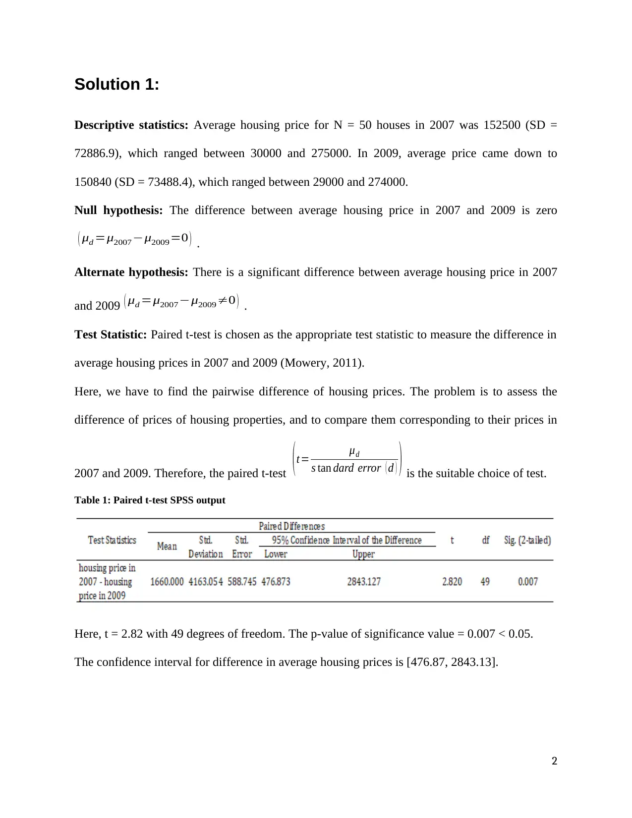
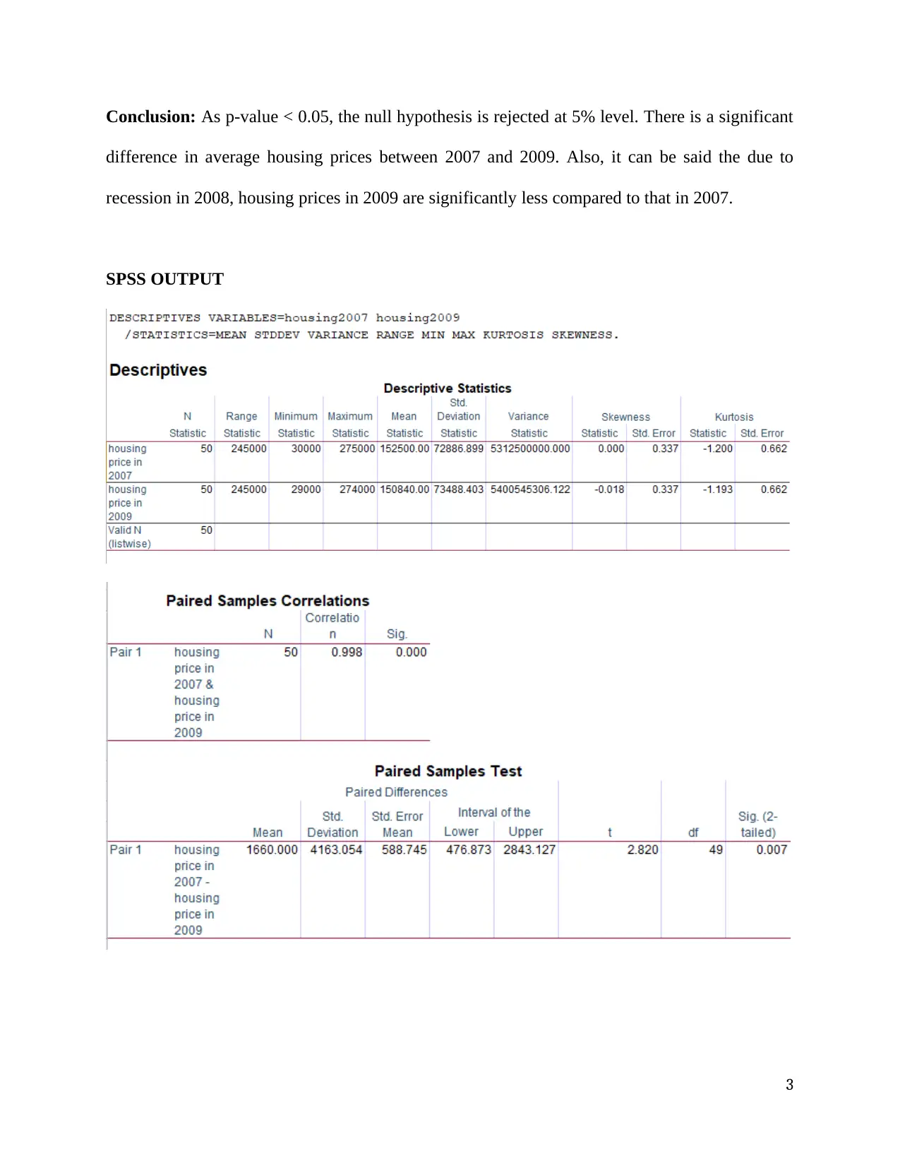
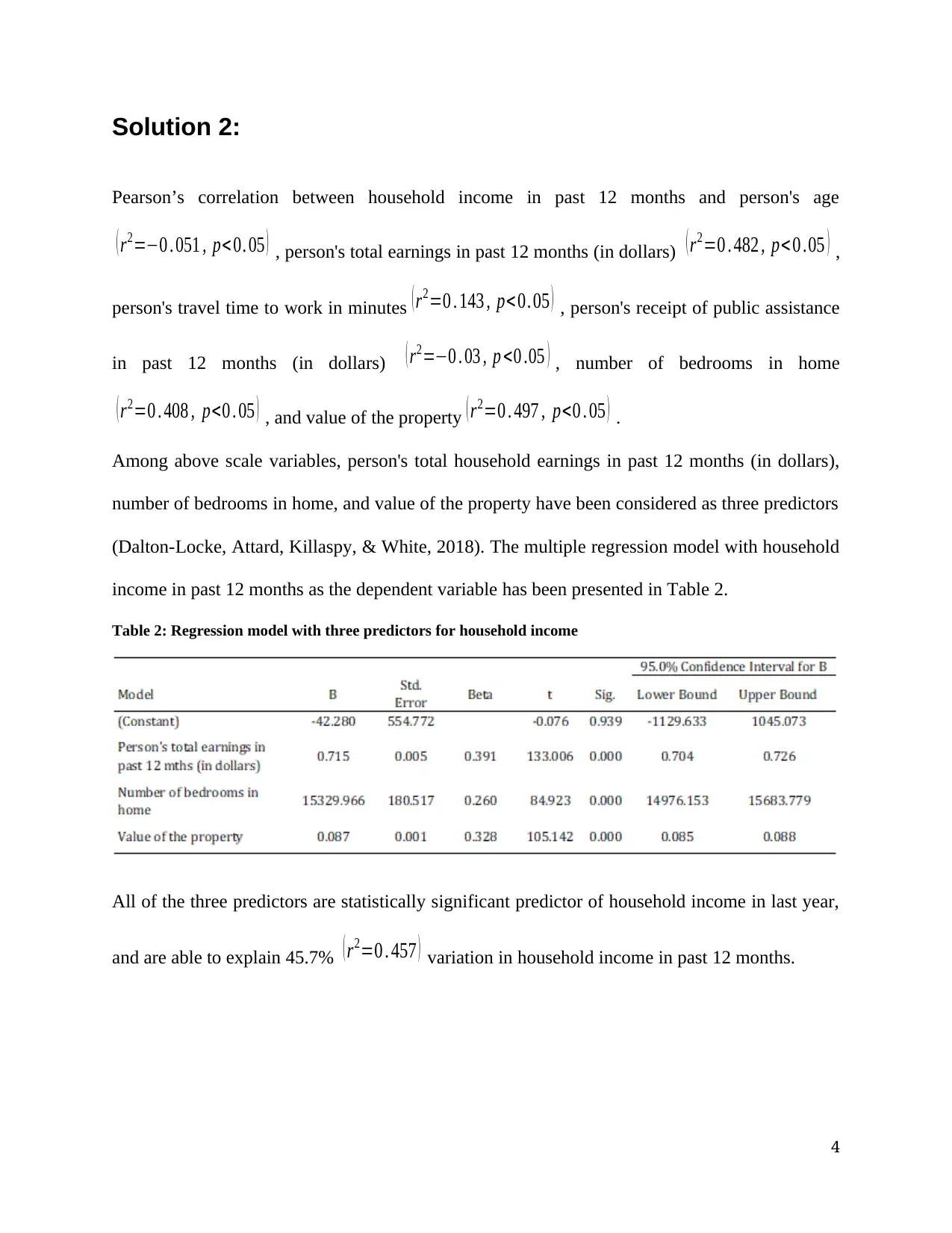
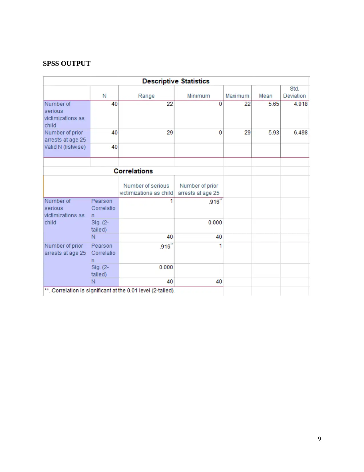
This document presents a comprehensive solution to a statistical analysis assignment (SOC 302), addressing multiple problems using various statistical methods. The solutions include paired t-tests to compare housing prices before and after a recession, Pearson's correlation to analyze relationships between variables like income and age, multiple regression to predict household income, independent t-tests to compare disciplinary problems in schools, two-way ANOVA to analyze the impact of prior arrests and community on sentence length, one-way ANOVA to compare hotel rates, and chi-square tests to examine the association between political affiliation and geographic regions. Each solution includes null and alternative hypotheses, the rationale for choosing the appropriate statistical test, descriptive statistics, SPSS output, and a final conclusion with statistical notation. The assignment covers a range of statistical concepts and their practical applications, providing a detailed analysis of each problem and its solution.

SOC 302 – Statistical Analysis
1

Solution 1:
Descriptive statistics: Average housing price for N = 50 houses in 2007 was 152500 (SD =
72886.9), which ranged between 30000 and 275000. In 2009, average price came down to
150840 (SD = 73488.4), which ranged between 29000 and 274000.
Null hypothesis: The difference between average housing price in 2007 and 2009 is zero
( μd =μ2007−μ2009=0 ) .
Alternate hypothesis: There is a significant difference between average housing price in 2007
and 2009 ( μd =μ2007−μ2009≠0 ) .
Test Statistic: Paired t-test is chosen as the appropriate test statistic to measure the difference in
average housing prices in 2007 and 2009 (Mowery, 2011).
Here, we have to find the pairwise difference of housing prices. The problem is to assess the
difference of prices of housing properties, and to compare them corresponding to their prices in
2007 and 2009. Therefore, the paired t-test ( t= μd
s tan dard error ( d ) ) is the suitable choice of test.
Table 1: Paired t-test SPSS output
Here, t = 2.82 with 49 degrees of freedom. The p-value of significance value = 0.007 < 0.05.
The confidence interval for difference in average housing prices is [476.87, 2843.13].
2

Conclusion: As p-value < 0.05, the null hypothesis is rejected at 5% level. There is a significant
difference in average housing prices between 2007 and 2009. Also, it can be said the due to
recession in 2008, housing prices in 2009 are significantly less compared to that in 2007.
SPSS OUTPUT
3

Solution 2:
Pearson’s correlation between household income in past 12 months and person's age
( r2=−0 . 051 , p< 0. 05 ) , person's total earnings in past 12 months (in dollars) ( r2=0 . 482 , p< 0 .05 ) ,
person's travel time to work in minutes ( r2=0 . 143 , p<0. 05 ) , person's receipt of public assistance
in past 12 months (in dollars) ( r2=−0 . 03 , p <0 .05 ) , number of bedrooms in home
( r2=0 . 408 , p<0 . 05 ) , and value of the property ( r2=0 . 497 , p<0 . 05 ) .
Among above scale variables, person's total household earnings in past 12 months (in dollars),
number of bedrooms in home, and value of the property have been considered as three predictors
(Dalton-Locke, Attard, Killaspy, & White, 2018). The multiple regression model with household
income in past 12 months as the dependent variable has been presented in Table 2.
Table 2: Regression model with three predictors for household income
All of the three predictors are statistically significant predictor of household income in last year,
and are able to explain 45.7% ( r2=0 . 457 ) variation in household income in past 12 months.
4

The regression equation is,
Household income in past 12 months = 0.087*Value of the property + 15329.97*Number of
bedrooms in home + 0.715*Person’s total earning in past 12 months – 42.28
Descriptive statistics: Average household income in past 12 months for N = 65535 persons is
75248.32 (SD = 78596.49). Average number of bedrooms is 2.96 (SD = 1.33), and average value
of property is 297022.27 (SD = 186131.26).
Null hypothesis: H0 : ( βi=0 ) where βi s are the slopes of the predictors.
Alternate hypothesis: H A ( βi≠0 ) where βi s are the slopes of the predictors.
Test Statistic: The chosen test statistic was t-statistic, where the values have been obtained from
SPSS output.
Value of the property: t-stat =
β1
SE ( β1 ) =105.14, p-value < 0.05.
Number of bedrooms in home: t-stat =
β2
SE ( β2 ) =84.92, p-value < 0.05.
Person’s total earning in past 12 months: t-stat =
β3
SE ( β 3 ) =133.0, p-value < 0.05.
Conclusion: There was enough statistical evidence to reject the null hypotheses, concluding that
the predictors are linearly related to the dependent variable.
5

SPSS OUTPUT
6

7

Solution 3:
Descriptive statistics: Average number of serious victimizations for N = 40 persons is 5.65 (SD
= 4.92), which ranged between 0 and 22. Average number of arrests by the age of 25 is 5.93 (SD
= 6.50), which ranged between 0 and 29.
Null hypothesis: H0 : ( r =0 ) : There is no correlation between the number of arrests by the age of
25 and number of serious victimization experiences.
Alternate hypothesis: H A : ( r≠0 ) : There is significant correlation between number of arrests by
the age of 25 and number of serious victimization experiences.
Test Statistic: The chosen test statistic was Pearson’s correlation coefficient, where the values
have been obtained from SPSS output. Both the variables are continuous variables, and there
association is measured by Pearson’s correlation coefficient (Emerson, 2015).
Pearson’s correlation coefficient = r=0. 916 , and p-value < 0.05.
Conclusion: There was enough statistical evidence to reject the null hypotheses, and the social
service provider concluding that there is a significant and positive (almost perfect positive)
correlation between number of arrests by the age of 25 and number of serious victimization
experiences.
8

SPSS OUTPUT
9

Solution 4:
Descriptive statistics: Average number of disciplinary problems for N = 150 students in school
A is 12.17 (SD =7.49). In school B, average number of disciplinary problems is 10.95 (SD =
6.53). Number of disciplinary problems in both the schools ranged between 0 and 25.
Null hypothesis: There is no difference between average number of disciplinary problems
between school A and school B.
Alternate hypothesis: There is no significant difference between average number of disciplinary
problems between school A and school B.
Test Statistic: Independent t-test is chosen as the appropriate test statistic to measure the
difference in average number of disciplinary problems between school A and school B (Kim,
2015).
Here, we have to find difference in number of disciplinary problems for two different schools.
The problem is to assess two samples from two different populations. Therefore, the independent
t-test is the suitable choice of test.
From Levene’s test, it was noted that the two samples have equal variances (F = 6.101, p < 0.05).
Hence for equal variances, t = 1.50 with 298 degrees of freedom. The p-value of significance
value = 0.134 > 0.05.
The confidence interval for difference in average housing prices is [-0.377, 2.817].
Conclusion: As p-value > 0.05, the null hypothesis failed to get rejected at 5% level. There is no
significant difference in number of disciplinary problems between school A and school B. Also,
10

the superintendent can conclude that eating and drinking less sugar does not reduce number of
disciplinary problems in students, and there is no point keeping the level down in school A. .
SPSS OUTPUT
11

Solution 5:
Descriptive statistics: Number of no prior arrests is 43, and at least 1 prior arrest is 57. People
from urban area are 45, and those from rural are 55 in number. No prior arrests from rural area
are 24, and from urban area are 19. Again, at least one prior arrest from rural area is 31, and from
urban area are 26.
Null hypotheses:
H01: Prior arrest history (Arrests) has equal impact on average sentence length.
H02: Both urban and rural defendants (UrbRur) have equal influence on average sentence length.
H03: Both the factors are independent and interaction effect between them is not present.
Alternate hypothesis:
HA1: Two prior arrest histories differ significantly in average sentence length.
HA1: Two defendant communities differ significantly in average sentence length.
HA3: The interaction effect between the two factors is significantly present.
Test Statistic: Two-way ANOVA (F-statistics) or factorial ANOVA is chosen as the appropriate
test statistic to measure the difference in average sentence length for the factors (George, &
Mallery, 2016).
Here, we have to find difference in average sentence length between the two states of each
factor. The problem is to compare two sample means for two factors, and their means for their
interaction also. Therefore, two-factor ANOVA is the suitable choice of test.
12

From Levene’s test, it was noted that variances of sentence length for the design: Intercept +
Arrests + UrbRur + Arrests * UrbRur are significantly unequal (F (3, 96) = 5.93, p < 0.05).
The two-way ANOVA implied with F = 4.21, and p-value = 0.008 < 0.05, that the model is
statistically significant.
All Possible Relations:
Prior arrest history (F = 9.47, p < 0.05) is noted to have significant impact on sentence length,
where it is able to explain only 9% variation in sentence length. Community of defendants
(UrbRur) is not statistically significant in differentiating between average sentence length (F =
0.005, p = 0.944). Post-hoc analysis revealed that average sentence length is significantly greater
by 11.6 units in case of at least one prior crime compared to no prior crime history.
Average service length is 8.12 (SE = 3.79) for rural area defendant with no prior arrest history.
Average service length is 13.26 (SE = 4.26) for urban area defendant with no prior arrest history.
Average service length is 25.13 (SE = 3.33) for rural area defendant with at least one prior arrest
history.
Average service length is 19.46 (SE = 3.64) for urban area defendant with at least one prior
arrest history.
The interaction of prior arrest history and community of defendants also has no significant
differentiating impact on sentence length (F = 2.05, p = 0.155).
Conclusion: The H01 null hypothesis gets rejected at 5% level. Null hypotheses H02 and H03
fail to get rejected at 5% level of significance. There is significant difference in average sentence
length between two positions of prior crime status, where prior crime is noted to have a negative
13

impact. Community has no significant differentiating impact, and interaction with prior crime
status also is found insignificant.
SPSS OUTPUT
14

15

16

Solution 6:
Descriptive statistics: In the sample of N = 160 people, 33.1% (N = 53) are from east region,
23.8% (N = 38) are from Midwest, and 43.1% (N = 69) people are from west. Distribution of
political affiliation reflected 56.9% republican (N = 91), 43.1% democrats (N = 69).
Null hypothesis: H0 : ( μ1=μ2=μ3 ) There is no difference between average hotel rates per night
among hotels in uptown, downtown, and midtown.
Alternate hypothesis: At least one place (uptown, downtown, or midtown) differs significantly
in average hotel rates per night.
Test Statistic: One-way ANOVA (F-statistics) is chosen as the appropriate test statistic to
measure the difference in average hotel rates per night among hotels in uptown, downtown, and
midtown.
Here, we have to find difference in average hotel rates per night among hotels in three places.
The problem is to compare three sample means; therefore, ANOVA is the suitable choice of test.
17

From Levene’s test, it was noted that the three samples have significantly unequal variances (F =
59.88, p < 0.05).
The one-way ANOVA implied with F =107.48, with total 224 degrees of freedom. The p-value
of significance value = 0.000 < 0.05.
Conclusion: As p-value < 0.05, the null hypothesis gets rejected at 5% level. There is significant
difference in average hotel rates per night among hotels in uptown, downtown, and midtown, and
the information is significant for tourism professional.
SPSS OUTPUT
18

Solution 7:
Descriptive statistics: In the sample of N = 160 people, 33.1% (N = 53) are from east region,
23.8% (N = 38) are from Midwest, and 43.1% (N = 69) people are from west. Distribution of
political affiliation reflected 56.9% republican (N = 91), 43.1% democrats (N = 69).
19

Null hypothesis: H0 : There is no association between political affiliation and geographic
regions.
Alternate hypothesis: There is significant association between political affiliation and
geographic regions.
Test Statistic: χ2
test of independence is chosen as the appropriate test statistic to measure the
association between political affiliation and geographic regions (Rana, & Singhal, 2015).
Here, we have to find association between two political affiliations and three geographic regions.
The problem is to find association between two nominal variables. Therefore, a cross tabulation
with Chi-square test is appropriate choice. .
The Chi-square test statistic implied with χ2
=0.164, with total 2 degrees of freedom. The
asymptotic p-value for significance = 0.921 > 0.05.
Conclusion: As p-value > 0.05, the null hypothesis failed to get rejected at 5% level. There is no
significant association between two political affiliations and three geographic regions. Hence, the
student can conclude that political affiliation of people is not affected by region.
SPSS OUTPUT
20

21

22

Solution 8:
Pearson’s correlation between games own this year and free throw percentages
( r2=0 . 961 , p< 0. 05 ) , having a rookie vs. veteran coach ( r2=0 . 388 , p< 0. 05 ) , person's travel time
to work in minutes ( r2=0 . 143 , p<0. 05 ) , games won during the previous season
( r2=0 . 995 , p< 0 .05 ) .
The multiple regression model with games own this year as the dependent variable has been
presented in Table 3.
Table 3: Regression model with three predictors for games own this year
All of the three predictors are statistically significant predictor of games own this year, and are
able to explain 99.1% ( r2=0 . 991 ) variation in games own this year.
The regression equation is,
Games own this year = 14.18* free throw percentages + 0.85* rookie vs. veteran coach +
1.0*games own last year – 13.75
23

Descriptive statistics: Average games own this year for N = 125 appearances of NBA teams is
52.35 (SD = 16.69). Average free throw percentages is 0.81 (SD = 0.09), and average number of
games won during the previous season is 53.79 (SD = 15.19). 33.6% (N = 42) teams had rookie
coaches, and in 66.4% (N = 83) matches teams had veteran coaches.
Null hypothesis: H0 : ( βi=0 ) where βi s are the slopes of the predictors.
Alternate hypothesis: H A ( βi≠0 ) where βi s are the slopes of the predictors.
Test Statistic: The chosen test statistic was t-statistic, where the values have been obtained from
SPSS output.
Free throw percentages: t-stat =
β1
SE ( β1 ) 2.38, p-value < 0.05.
Rookie vs. veteran coach: t-stat =
β2
SE ( β2 ) = 2.52, p-value < 0.05.
Games own last year: t-stat =
β3
SE ( β 3 ) =28.89, p-value < 0.05.
Conclusion: There was enough statistical evidence to reject the null hypotheses, concluding that
the predictors are linearly related to the dependent variable and successfully predict the games
own this year.
24

SPSS OUTPUT
25

26

Solution 9:
a. Factorial ANOVA
Researchers are interested in whether a person's interest in politics is dependent on their level of
education and gender. They occasionally asked the participants of the study and questioned their
interest in politics. Interest in politics was ranked between 0 and 100, the higher the score, the
more interest in politics. The researchers divided the participants by gender (male = 1 / female =
0), and then training (school =1 / college = 2 / university = 3). The response variable is "interest
in politics" (scale variable) and two predictor variables are "gender" and "education" (nominal
factors).
Factorial ANOVA is applicable to this scenario in lieu of the followings,
 Response variable was measured at the continuous level.
 Two predictor variables consist of two or more categorical groups.
 Observations were independent (Rouder, Engelhardt, McCabe, & Morey, 2016).
Null hypotheses:
H01: Both the genders have equal average interest in politics.
H02: Trainings of the participants have equal influence on average interest in politics.
H03: Both the factors are independent and interaction effect between them is not present.
Alternate hypothesis:
HA1: Both the genders differ significantly for their average interest in politics.
HA1: Trainings of the participants have significant influence on average interest in politics, and
one of the trainings has significantly different average level of interest in politics.
HA3: The interaction effect between the two factors is significantly present.
27

b. Correlations
The relationship between drinking coffee and the number of hours staying awake is measured.
Sample data was collected from N = 75 participants. Number of cups of coffee consumed in a
cup of 100 ml was noted. Next, information was collected about total hours of sleep in last 7
days. From there total hours of awake were evaluated.
Correlation Analysis is applicable as,
Both the data are continuous or scale type, and their association can be evaluated using
correlation.
Null hypothesis: There is no statistical relationship between number of hours staying awake and
drinking coffee.
Alternative hypothesis: There is a statistically significant relationship between number of hours
staying awake and drinking coffee.
c. Chi-square test of independence
A sample of 1000 voter participated in the survey. Respondents were classified by gender (male
or female) and by political orientation (Republic, Democratic or independent). The results are
listed in the table below.
Republican Democrats Independent
Male 250 300 40 590
Female 200 150 60 410
Total 450 450 100 1000
Voting Preferences
Row total
28

Is there a difference between the sexes over political orientation? What is the difference between
men's preferences and women's preferences?
The chi square test of independence test is applicable as the two categorical variables are from a
single population. We have to determine whether there is a significant association between
gender and voting preferences.
Null hypothesis: H0 : There is no association between political affiliation and two sexes.
Alternate hypothesis: There is significant association between political affiliation and two
sexes.
d. Multiple linear regression
Problem Statement: Assessment of the effect of BMI, age (a continuous variable, measured in
years), gender (male = 1/female = 0), and treatment for hypertension (yes = 1 /no =0) as potential
confounders on systolic blood pressure. The problem accounts for using multiple linear
regression analysis (Anghelache, Manole, & Anghel, 2015).
Systolic pressure is a continuous and scale variable, which is estimated by one continuous (age)
and two categorical variables with specified reference categories. Hence, multiple regression
model estimating systolic blood pressure is appropriate considering historical knowledge of
linear relationship between the dependent and independent variables. The normality of the
residuals has to be checked.
Null hypothesis: H0 : ( βi=0 ) where βi s are the slopes of the predictors, implying no linear
relation between the dependent and the predictor.
Alternate hypothesis: H A ( βi≠0 ) where βi s are the slopes of the predictors, implying
significant linear relation.
29

References
Anghelache, C., Manole, A., & Anghel, M. G. (2015). Analysis of final consumption and gross
investment influence on GDP–multiple linear regression model. Theoretical and Applied
Economics, 22(3), 604.
Dalton-Locke, C., Attard, R., Killaspy, H., & White, S. (2018). Predictors of quality of care in
mental health supported accommodation services in England: a multiple regression
modelling study. BMC psychiatry, 18(1), 344.
Emerson, R. W. (2015). Causation and Pearson's correlation coefficient. Journal of visual
impairment & blindness, 109(3), 242-244.
George, D., & Mallery, P. (2016). General Linear Models: Two-Way ANOVA. In IBM SPSS
Statistics 23 Step by Step (pp. 183-190). Routledge.
Kim, T. K. (2015). T test as a parametric statistic. Korean journal of anesthesiology, 68(6), 540.
Mowery, B. D. (2011). The paired t-test. Pediatric nursing, 37(6), 320.
Rana, R., & Singhal, R. (2015). Chi-square test and its application in hypothesis testing. Journal
of the Practice of Cardiovascular Sciences, 1(1), 69.
Rouder, J. N., Engelhardt, C. R., McCabe, S., & Morey, R. D. (2016). Model comparison in
ANOVA. Psychonomic Bulletin & Review, 23(6), 1779-1786.
30