Data Classification Project: University Name, Subject Code Analysis

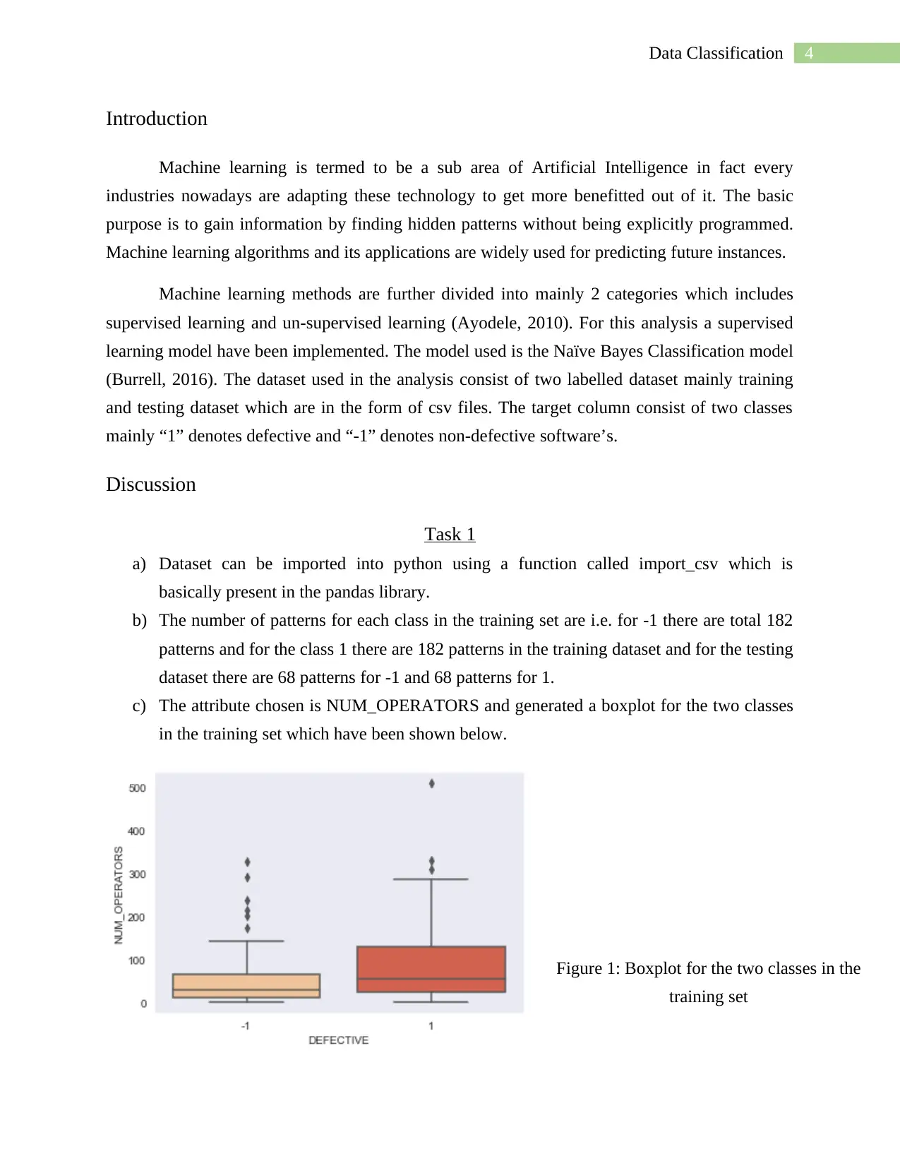
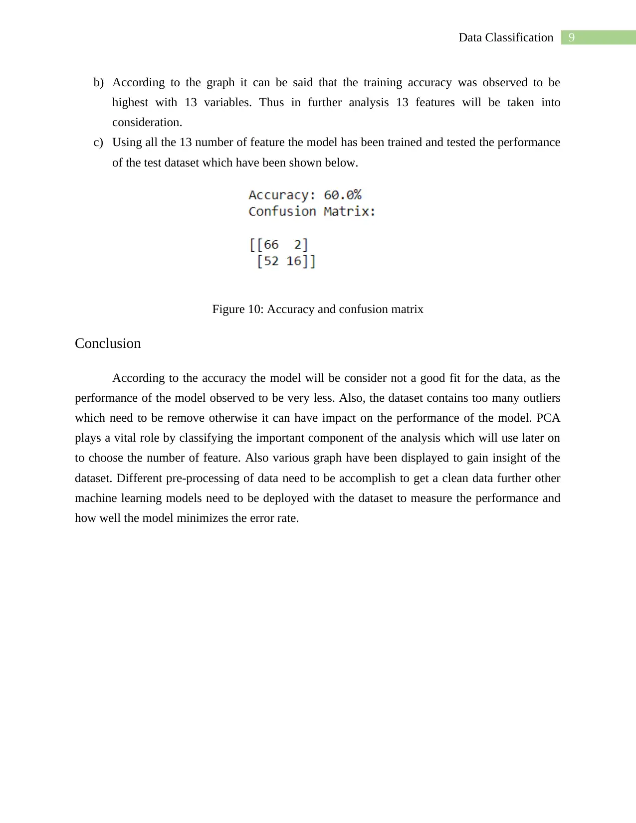
This project presents a comprehensive analysis of software defect prediction using machine learning techniques. The student implemented a Naive Bayes classification model to analyze a dataset containing static code metrics. The project includes data preprocessing, exploratory data analysis (EDA) with visualizations like boxplots and scatter plots, and dimensionality reduction using Principal Component Analysis (PCA). The analysis involved splitting the data into training and testing sets, building and evaluating the Naive Bayes model, and assessing its performance using accuracy, classification reports, and confusion matrices. The project also explored the impact of different features on model accuracy. The conclusion highlights the model's performance, the presence of outliers, and the importance of PCA for feature selection, along with suggestions for future improvements, such as employing other machine learning models and data preprocessing techniques to enhance the prediction accuracy. The project is a practical application of machine learning for software quality assessment.

Running head: DATA CLASSIFICATION
Data Classification
Student Name:
Student ID:
University Name:
Subject Code:

2Data Classification
Executive Summary
Machine learning is termed to be a sub area of Artificial Intelligence in fact every industries
nowadays are adapting these technology to get more benefitted out of it. The basic purpose is to
gain information by finding hidden patterns without being explicitly programmed. Machine
learning algorithms and its applications are widely used for predicting future instances and for
forecasting. In this analysis one vital algorithm will be used for the classification purpose and a
dataset will be feed to the model where for each function contains the static code metrics which
generally consist a software system. Various types of analysis and visualization will be done
over the data to get better insight. Also using a supervised machine learning model prediction
will be applied over the dataset. And at the end few conclusion regarding the dataset, analysis
and the performance of the model will be concluded with some future scope.

3Data Classification
Table of Contents
Executive Summary.........................................................................................................................2
Introduction......................................................................................................................................4
Discussion........................................................................................................................................4
Task 1...........................................................................................................................................4
Task 2...........................................................................................................................................5
Task 3...........................................................................................................................................8
Task 4...........................................................................................................................................8
Conclusion.......................................................................................................................................9
References......................................................................................................................................10

4Data Classification
Introduction
Machine learning is termed to be a sub area of Artificial Intelligence in fact every
industries nowadays are adapting these technology to get more benefitted out of it. The basic
purpose is to gain information by finding hidden patterns without being explicitly programmed.
Machine learning algorithms and its applications are widely used for predicting future instances.
Machine learning methods are further divided into mainly 2 categories which includes
supervised learning and un-supervised learning (Ayodele, 2010). For this analysis a supervised
learning model have been implemented. The model used is the Naïve Bayes Classification model
(Burrell, 2016). The dataset used in the analysis consist of two labelled dataset mainly training
and testing dataset which are in the form of csv files. The target column consist of two classes
mainly “1” denotes defective and “-1” denotes non-defective software’s.
Discussion
Task 1
a) Dataset can be imported into python using a function called import_csv which is
basically present in the pandas library.
b) The number of patterns for each class in the training set are i.e. for -1 there are total 182
patterns and for the class 1 there are 182 patterns in the training dataset and for the testing
dataset there are 68 patterns for -1 and 68 patterns for 1.
c) The attribute chosen is NUM_OPERATORS and generated a boxplot for the two classes
in the training set which have been shown below.
Figure 1: Boxplot for the two classes in the
training set

5Data Classification
d) To build scatter plot two feature have been used from the dataset which includes
LOC_BLANK and NUM_OPERATORS and have been shown below.
Figure 2: Scatter plot of one feature with another
e) For splitting of dataset train_test_split function has been used to split the original training
data into trained validation set in the ratio of 45:55.
Task 2
a) PCA analysis are generally used to dimension reduction purpose for the dataset if the
dataset is too large. It is use to convert correlated variables to a set of uncorrelated
variables using orthogonal transformation (Murphy, 2012). It is done to examine the
interrelations among the set of variables. Mainly this process can be achieved using
Feature Elimination and Feature Extraction (Zhang, Peña & Robles, 2009). Here PCA
analysis have been performed and it has been found that the captured variance by each
Principals components are:
[7.36900855e-01 7.84966264e-02 6.84054476e-02 3.97040308e-02 3.32871877e-02
1.79152798e-02 1.39358457e-02 5.16537011e-03 2.95944079e-03 2.19399041e-03
8.09787283e-04 1.53774840e-04 7.23634635e-05]
b) In simple to plot the eigenvalues of factors or PCA scree plot is used. It determines the
number of principal component which is crucial in the principal component analysis.
Basically it visualize the variance captured by each of the principal components. Below
the scree plot have been shown.

6Data Classification
Figure 3: Scree plot
c) PCA of training and test dataset has been shown below-
d)
Two subplots have been plotted in one figure i.e., one for the training data in the PC1 and
PC2 projection space and label the data in the picture according to its class and the other
one for the test data in the same PCA space and label the data in the picture according to
its class which have been shown below. The figure below shows the scatter plot PC1 vs.
PC2.
Figure 4: PC1 and PC2 for training
data
Figure 5: PC1 and PC2 for test data

7Data Classification
Figure 6: Scatter plot of PC1 and PC2 for training data
Figure 7: Scatter plot of PC1 and PC2 for testing data

8Data Classification
Task 3
Naïve Bayes Classification model are generally used to classify the target attributes also
to predict the future instances (Snoek, Larochelle & Adams, 2012). It is consider to be a
probabilistic machine learning model which is useful for classification purposes. It is totally
based on Bayes’ Theorem which concludes that the model is a collection of classification
algorithms. There are various kind of Naïve Bayes classifiers available and particularly for this
analysis Gaussian Naive Bayes model has been implemented for the classification of defective
software’s (Tramèr et al., 2016).
The below figure shows the accuracy, classification report and the confusion matrix of
the model.
Figure 8: Performance of Naive Bayes classification model
Task 4
a) In this section 13 different Naïve Bayes Classification models were built with 13
different feature using the training set (II) and the validation set which was built in
earlier. The accuracy of both the training (II) and validation set have been reported and an
accuracy vs. number of feature graph has been shown below.
Figure 9: Accuracy vs. Feature graph

9Data Classification
b) According to the graph it can be said that the training accuracy was observed to be
highest with 13 variables. Thus in further analysis 13 features will be taken into
consideration.
c) Using all the 13 number of feature the model has been trained and tested the performance
of the test dataset which have been shown below.
Figure 10: Accuracy and confusion matrix
Conclusion
According to the accuracy the model will be consider not a good fit for the data, as the
performance of the model observed to be very less. Also, the dataset contains too many outliers
which need to be remove otherwise it can have impact on the performance of the model. PCA
plays a vital role by classifying the important component of the analysis which will use later on
to choose the number of feature. Also various graph have been displayed to gain insight of the
dataset. Different pre-processing of data need to be accomplish to get a clean data further other
machine learning models need to be deployed with the dataset to measure the performance and
how well the model minimizes the error rate.

10Data Classification
References
Ayodele, T. O. (2010). Types of machine learning algorithms. New advances in machine
learning, 19-48.
Burrell, J. (2016). How the machine ‘thinks’: Understanding opacity in machine learning
algorithms. Big Data & Society, 3(1), 2053951715622512.
Murphy, K. P. (2012). Machine learning: a probabilistic perspective. MIT press.
Snoek, J., Larochelle, H., & Adams, R. P. (2012). Practical bayesian optimization of machine
learning algorithms. In Advances in neural information processing systems (pp. 2951-
2959).
Tramèr, F., Zhang, F., Juels, A., Reiter, M. K., & Ristenpart, T. (2016). Stealing machine
learning models via prediction apis. In 25th {USENIX} Security Symposium
({USENIX} Security 16) (pp. 601-618).
Zhang, M. L., Peña, J. M., & Robles, V. (2009). Feature selection for multi-label naive Bayes
classification. Information Sciences, 179(19), 3218-3229.