Mechanical Engineering Homework: Spring Assemblage Analysis

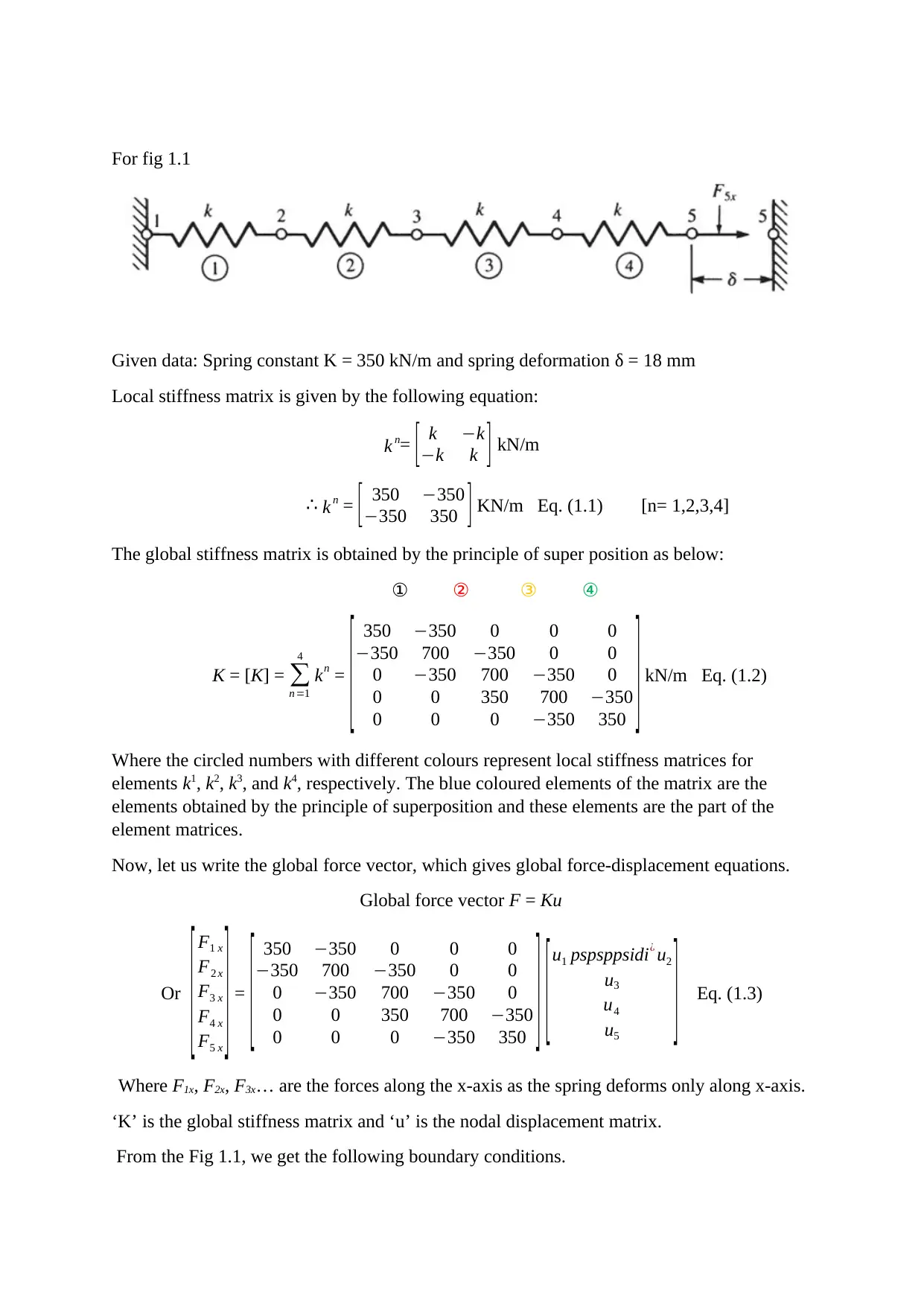
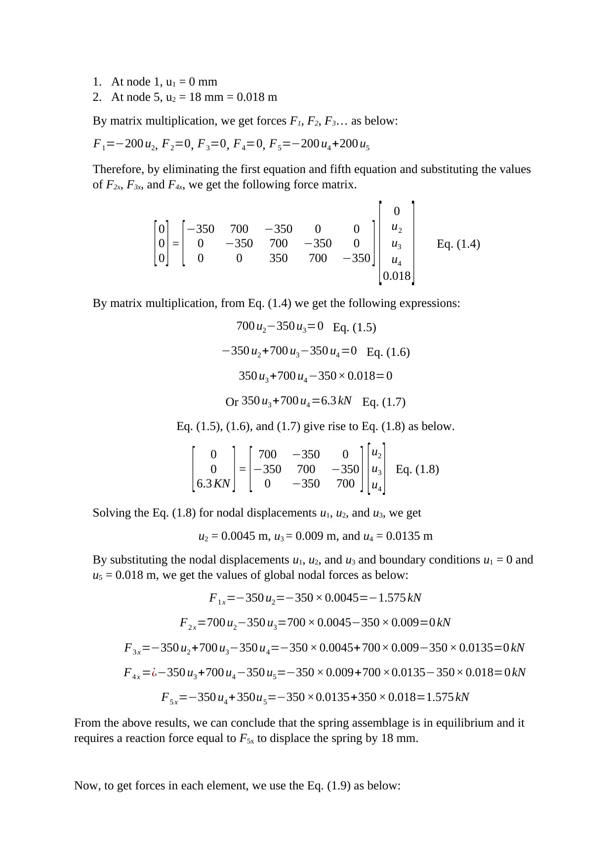
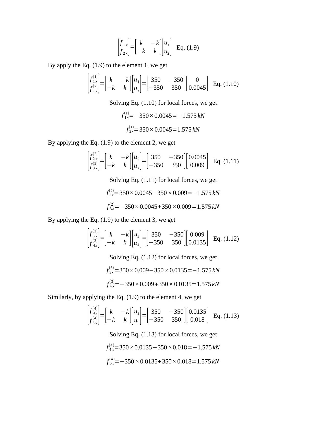
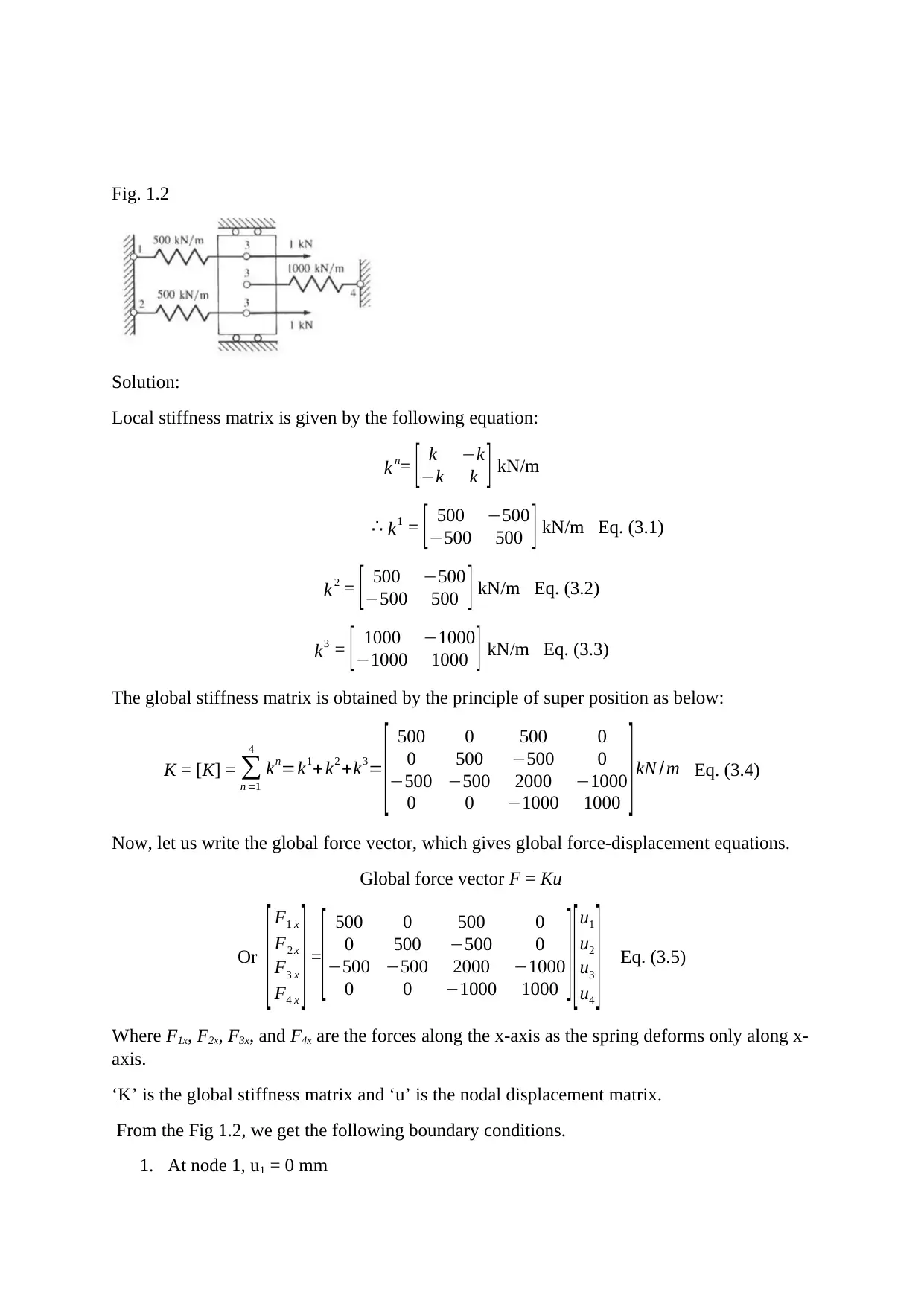
This document presents detailed solutions for spring assemblage analysis problems, crucial in mechanical engineering. The solutions encompass the calculation of local and global stiffness matrices, nodal displacements, and forces within the spring elements. The document analyzes three different spring assemblage configurations (Fig 1.1, Fig 1.2, and Fig 1.3), providing step-by-step calculations for each, including boundary conditions, matrix multiplication, and the application of relevant equations (Eq. 1.1 to 3.10). The solutions demonstrate how to determine nodal forces, element forces, and overall equilibrium of the spring systems. The analysis involves the use of superposition principles and the application of force-displacement relationships to derive the necessary equations for solving the problems. The document effectively illustrates the process of spring assemblage analysis, offering a comprehensive understanding of the underlying concepts and methodologies.

For fig 1.1
Given data: Spring constant K = 350 kN/m and spring deformation δ = 18 mm
Local stiffness matrix is given by the following equation:
k n= [ k −k
−k k ] kN/m
∴ k n = [ 350 −350
−350 350 ] KN/m Eq. (1.1) [n= 1,2,3,4]
The global stiffness matrix is obtained by the principle of super position as below:
① ② ③ ④
K = [K] = ∑
n =1
4
kn =
[ 350 −350 0 0 0
−350 700 −350 0 0
0 −350 700 −350 0
0 0 350 700 −350
0 0 0 −350 350 ] kN/m Eq. (1.2)
Where the circled numbers with different colours represent local stiffness matrices for
elements k1, k2, k3, and k4, respectively. The blue coloured elements of the matrix are the
elements obtained by the principle of superposition and these elements are the part of the
element matrices.
Now, let us write the global force vector, which gives global force-displacement equations.
Global force vector F = Ku
Or
[ F1 x
F2 x
F3 x
F4 x
F5 x
] =
[ 350 −350 0 0 0
−350 700 −350 0 0
0 −350 700 −350 0
0 0 350 700 −350
0 0 0 −350 350 ] [u1 pspsppsidi¿ u2
u3
u4
u5
] Eq. (1.3)
Where F1x, F2x, F3x… are the forces along the x-axis as the spring deforms only along x-axis.
‘K’ is the global stiffness matrix and ‘u’ is the nodal displacement matrix.
From the Fig 1.1, we get the following boundary conditions.

1. At node 1, u1 = 0 mm
2. At node 5, u2 = 18 mm = 0.018 m
By matrix multiplication, we get forces F1, F2, F3… as below:
F1=−200 u2, F2=0, F3=0, F4=0, F5=−200 u4 +200 u5
Therefore, by eliminating the first equation and fifth equation and substituting the values
of F2x, F3x, and F4x, we get the following force matrix.
[ 0
0
0 ] = [−350 700 −350 0 0
0 −350 700 −350 0
0 0 350 700 −350 ] [ 0
u2
u3
u4
0.018 ] Eq. (1.4)
By matrix multiplication, from Eq. (1.4) we get the following expressions:
700 u2−350 u3=0 Eq. (1.5)
−350 u2 +700 u3−350 u4 =0 Eq. (1.6)
350 u3 +700 u4 −350× 0.018=0
Or 350 u3 +700 u4 =6.3 kN Eq. (1.7)
Eq. (1.5), (1.6), and (1.7) give rise to Eq. (1.8) as below.
[ 0
0
6.3 KN ] = [ 700 −350 0
−350 700 −350
0 −350 700 ] [u2
u3
u4 ] Eq. (1.8)
Solving the Eq. (1.8) for nodal displacements u1, u2, and u3, we get
u2 = 0.0045 m, u3 = 0.009 m, and u4 = 0.0135 m
By substituting the nodal displacements u1, u2, and u3 and boundary conditions u1 = 0 and
u5 = 0.018 m, we get the values of global nodal forces as below:
F1 x=−350 u2=−350 × 0.0045=−1.575 kN
F2 x=700 u2−350 u3=700 × 0.0045−350 × 0.009=0 kN
F3 x=−350 u2 +700 u3−350 u4=−350 × 0.0045+700× 0.009−350 × 0.0135=0 kN
F4 x =¿−350 u3 +700 u4 −350 u5=−350 × 0.009+700 ×0.0135−350× 0.018=0 kN
F5 x=−350 u4 +350u5=−350 ×0.0135+350 × 0.018=1.575 kN
From the above results, we can conclude that the spring assemblage is in equilibrium and it
requires a reaction force equal to F5x to displace the spring by 18 mm.
Now, to get forces in each element, we use the Eq. (1.9) as below:

[f 1 x
f 2 x ]= [ k −k
−k k ] [u1
u2 ] Eq. (1.9)
By apply the Eq. (1.9) to the element 1, we get
[ f 1 x
(1)
f 1 x
(2) ]= [ k −k
−k k ] [ u1
u2 ] = [ 350 −350
−350 350 ][ 0
0.0045 ] Eq. (1.10)
Solving Eq. (1.10) for local forces, we get
f 1 x
(1)=−350× 0.0045=−1.575 kN
f 2 x
(1)=350× 0.0045=1.575 kN
By applying the Eq. (1.9) to the element 2, we get
[ f 2 x
(2)
f 3 x
(2) ]= [ k −k
−k k ] [ u2
u3 ]= [ 350 −350
−350 350 ][ 0.0045
0.009 ] Eq. (1.11)
Solving Eq. (1.11) for local forces, we get
f 2 x
(2)=350× 0.0045−350 × 0.009=−1.575 kN
f 3 x
(2)=−350× 0.0045+350 ×0.009=1.575 kN
By applying the Eq. (1.9) to the element 3, we get
[f 3 x
(3)
f 4 x
(3) ]=[ k −k
−k k ] [u3
u4 ]=[ 350 −350
−350 350 ][ 0.009
0.0135 ] Eq. (1.12)
Solving Eq. (1.12) for local forces, we get
f 3 x
(3)=350× 0.009−350 × 0.0135=−1.575 kN
f 4 x
(3)=−350 ×0.009+350 × 0.0135=1.575 kN
Similarly, by applying the Eq. (1.9) to the element 4, we get
[ f 4 x
(4)
f 5 x
(4) ] = [ k −k
−k k ] [ u4
u5 ] = [ 350 −350
−350 350 ][ 0.0135
0.018 ] Eq. (1.13)
Solving Eq. (1.13) for local forces, we get
f 4 x
(4 )=350 ×0.0135−350 ×0.018=−1.575 kN
f 5 x
(4 )=−350 × 0.0135+ 350× 0.018=1.575 kN

Fig. 1.2
Solution:
Local stiffness matrix is given by the following equation:
k n= [ k −k
−k k ] kN/m
∴ k1 = [ 500 −500
−500 500 ] kN/m Eq. (3.1)
k 2 = [ 500 −500
−500 500 ] kN/m Eq. (3.2)
k3 = [ 1000 −1000
−1000 1000 ] kN/m Eq. (3.3)
The global stiffness matrix is obtained by the principle of super position as below:
K = [K] = ∑
n =1
4
kn=k1+ k2 +k3=
[ 500 0 500 0
0 500 −500 0
−500 −500 2000 −1000
0 0 −1000 1000 ]kN /m Eq. (3.4)
Now, let us write the global force vector, which gives global force-displacement equations.
Global force vector F = Ku
Or
[ F1 x
F2 x
F3 x
F4 x
] =
[ 500 0 500 0
0 500 −500 0
−500 −500 2000 −1000
0 0 −1000 1000 ] [u1
u2
u3
u4
] Eq. (3.5)
Where F1x, F2x, F3x, and F4x are the forces along the x-axis as the spring deforms only along x-
axis.
‘K’ is the global stiffness matrix and ‘u’ is the nodal displacement matrix.
From the Fig 1.2, we get the following boundary conditions.
1. At node 1, u1 = 0 mm

2. At node 2, u2 = 0 mm
3. At node 4, u4 = 0 mm
4. F3x = 2 kN
Therefore, substituting u1, u2 and u4 and solving the third row of the Eq. (3.5) for u3 and we
get
[ F1 x
F2 x
2
F4 x
] =
[ 500 0 500 0
0 500 −500 0
−500 −500 2000 −1000
0 0 −1000 1000 ] [ 0
0
u3
0 ] Eq. (3.6)
2=2000u3
Or the nodal displacement at node 3, u3=0.001m
Substituting u1, u2, u3 and u4 in Eq. (3.5) and solving for the forces F1x, F2x, F3x, and F4x, we
get
[ F1 x
F2 x
F3 x
F4 x
] =
[ 500 0 500 0
0 500 −500 0
−500 −500 2000 −1000
0 0 −1000 1000 ][ 0
0
0.001
0 ]
Force at node 1 F1 x=−500 × ( 0.001 ) =−0.5 kN
Force at node 2 F2 x=−500 × ( 0.001 ) =−0.5 kN
Force at node 3 F3 x=2000 × ( 0.001 ) =2 kN
Force at node 4 F4 x =−1000× ( 0.001 ) =−1 kN
From the above results, we can conclude that the spring assemblage is in equilibrium.
Now, to get forces in each element, we use the Eq. (3.7) as below:
[f 1 x
f 2 x ]= [ k −k
−k k ] [u1
u2 ] Eq. (3.7)
Apply the Eq. (3.7) to the element 1, we get
[ f 1 x
(1)
f 3 x
(1) ]= [ k −k
−k k ] [ u1
u2 ] = [ 500 −500
−500 500 ][ 0
0.001 ] Eq. (3.8)
Solving Eq. (3.7) for local forces, we get
f 1 x
(1)=−500× (−0.001 )=−0.5 k N
f 3 x
(1)=500 × ( 0.001 ) =0.5 k N
Apply the Eq. (3.7) to the element 2, we get

[f 2 x
(2)
f 3 x
(2) ]= [ k −k
−k k ] [u1
u2 ]= [ 500 −500
−500 500 ][ 0
0.001 ] Eq. (3.9)
Solving Eq. (3.8) for local forces, we get
f 2 x
(2)=−500× ( 0.001 )=−0.5 kN
f 3 x
(2)=500× ( 0.001 )=0.5 k N
Apply the Eq. (3.7) to the element 3, we get
[ f 3 x
(3)
f 4 x
(3) ] =[ k −k
−k k ] [ u1
u2 ]= [ 1000 −1000
−1000 1000 ][ 0.001
0 ] Eq. (3.10)
Solving Eq. (3.9) for local forces, we get
f 3 x
(3)=1000× ( 0.001 )=1 kN
f 4 x
(3)=−1000 × ( 0.001 ) =−1k N
Fig. 1.3
Solution:
Local stiffness matrix is given by the following equation:
k n= [ k −k
−k k ] N/m
∴ k1 = [ 400 −400
−400 400 ] N/m Eq. (2.1)
k 2 = [ 400 −400
−400 400 ] KN/m Eq. (2.2)
The global stiffness matrix is obtained by the principle of super position as below:
K = [K] = ∑
n =1
4
kn=k1+ k2= [ 400 −400 0
−400 800 −400
0 −400 400 ] N /m Eq. (2.3)
Now, let us write the global force vector, which gives global force-displacement equations.

Global force vector F = Ku
Or [ F1 x
F2 x
F3 x ] =
[ 400 −400 0
−400 800 −400
0 −400 400 ] [u1
u2
u3 ] Eq. (2.4)
Where F1x, F2x, and F3x are the forces along the x-axis as the spring deforms only along x-
axis.
‘K’ is the global stiffness matrix and ‘u’ is the nodal displacement matrix.
From the Fig 1.3, we get the following boundary conditions.
5. At node 1, u1 = 0 mm
6. F1x = 100 N
7. F2x = −¿200 N
Therefore, by eliminating the first equation and substituting the values of F1x, F2x, and u1, we
get the following force matrix.
[ 100
−200 ]=[ 800 −400
−400 400 ] [u2
u3 ] Eq. (2.5)
By matrix multiplication, from Eq. (2.5) we get the following expressions:
800 u2−400 u3=100 Eq. (2.6)
−400u2+ 400 u3=−200 Eq. (2.7)
Solving Eq. (2.6) and (2.7) for u2 and u3, we get
u2=−0.25 m and u2=−0.75 m
By substituting the nodal displacements u2 and u3 and boundary conditions u1 = 0,
u2=−0.25 m and u2=−0.75 in Eq. (2.4), we get the values of global nodal forces as below:
[ F1 x
F2 x
F3 x ] =
[ 400 −400 0
−400 800 −400
0 −400 400 ] [ 0
−0.25
−0.75 ] Eq. (2.8)
Solving Eq. (2.8) F1x, F2x, and F3x, we get
Force at node 1 F1 x=−400×(−0.25)=100 N
Force at node 2 F2 x=800 × ( −0.25 ) +(−400)×(−0.75)=100 N
Force at node 3 F3 x=−400× (−0.25 ) +400× (−0.75 ) =−200 N
From the above results, we can conclude that the spring assemblage is in equilibrium.
Now, to get forces in each element, we use the Eq. (2.9) as below:
[f 1 x
f 2 x ]= [ k −k
−k k ] [u1
u2 ] Eq. (2.9)

Apply the Eq. (2.9) to the element 1, we get
[f 1 x
(1)
f 1 x
(2) ]= [ k −k
−k k ] [u1
u2 ]= [ 400 −400
−400 400 ][ 0
−0.25 ] Eq. (2.10)
Solving Eq. (2.10) for local forces, we get
f 1 x
(1)=−400 × (−0.25 )=100 N
f 2 x
(1)=400 × (−0.25 )=−100 N
Similarly, apply the Eq. (2.9) to the element 2, we get
[ f 2 x
(2)
f 3 x
(2) ]= [ k −k
−k k ] [ u1
u2 ] = [ 400 −400
−400 400 ][−0.25
−0.75 ] Eq. (2.11)
Solving Eq. (2.11) for local forces, we get
f 2 x
(2)=400 × (−0.25 )+(−400)× (−0.75 )=200 N
f 3 x
(2)=−400 × ( −0.25 ) +( 400) × ( −0.75 ) =−200 N