Comprehensive Data Analysis Report Using SPSS: Research Findings
VerifiedAdded on 2020/04/21
|19
|6803
|499
Report
AI Summary
This report presents a quantitative data analysis using SPSS to address research questions regarding young people's perceptions of violence, abuse, and control in relationships. The analysis includes 40 variables (4 nominal and 36 ordinal) from a sample of 120 participants. The report details the methodology, including descriptive statistics, cross-tabulations, linear regression, and independent t-tests. Findings are presented with tables and graphs, and interpretations are provided. The study examines relationships between variables such as age, gender, and mean scores of IPVAS-r subscales (control, abuse, violence) and Marlowe-Crowne social desirability. The report concludes with a discussion of the key findings and their implications.

Running head: DATA ANALYSIS WITH SPSS
Data Analysis with SPSS
Name of the Student:
Name of the University:
Author’s Note:
Data Analysis with SPSS
Name of the Student:
Name of the University:
Author’s Note:
Paraphrase This Document
Need a fresh take? Get an instant paraphrase of this document with our AI Paraphraser

DATA ANALYSIS WITH SPSS 1
Executive Summary
The report elaborates the data analysis of the participants’ data incorporated by SPSS. The data is analyzed and properly interpreted.
The SPSS analyzed data is reported with tables and graphs with valid interpretation. The relationship between 40 variables (4 nominal
and 36 ordinal) of 120 frequencies are reported and verified. We applied cross value summary with cross tab function, multiple R-
square by linear regression and summary by descriptive statistics. The conclusions and discussions are delivered along with
calculation.
DATA ANALYSIS WITH SPSS 2
Contents
Background and Introduction:-....................................................................................................................................................................3
Research Questions:-...................................................................................................................................................................................3
Findings, Calculation and Discussion:-.......................................................................................................................................................3
Crosstabs1................................................................................................................................................................................................3
Descriptive1.............................................................................................................................................................................................6
Frequency Tables.....................................................................................................................................................................................7
Descriptive2.............................................................................................................................................................................................8
Crosstabs2................................................................................................................................................................................................8
Linear Regression..................................................................................................................................................................................12
Independent-T test:-...............................................................................................................................................................................16
Conclusion:-...............................................................................................................................................................................................17
Annotated Bibliography:-..........................................................................................................................................................................18
⊘ This is a preview!⊘
Do you want full access?
Subscribe today to unlock all pages.
Trusted by 1+ million students worldwide
DATA ANALYSIS WITH SPSS 3
Background and Introduction:-
In this report, we have done quantitative data analysis report using SPSS in order to answer specific research questions. This
report will include a total number of 40 data variables of 120 frequencies. We have would write the background section, an account of
the process of analysis and discussion of the findings. These are supported by tables and charts as per needed. We have calculated the
appropriate descriptive statistics including dispersion and central tendency to describe participants and the relationships they are
engaging in. We have selected visual observations of tables and graphs to display the information. The mean results for the IPVAS-r
subscales (control, abuse, violence) are labeled as “MeanAbuse”, “MeanViolence” and “MeanControl”. The summary statistics of
MCSDS and IPVASr are calculated. The regression analysis between predictor identifier and Mean scores including Marlowe-Crowne
score of desirability are calculated and their results are interpreted to test the association.
Gender, Age, Ethnicity, Relationship Status and Sexual Orientation are nominal data. Rests of data are categorical. We have
scaled the data by Likert scale. Both of the qualitative and quantitative data are analyzed simultaneously.
Research Questions:-
The overall research questions of the report are:
1. To what extent do young people agree with the use of violence, abuse and control in relationships?
2. What kind of relationships are young people engaging in?
3. Find the descriptive statistics, totals, percentages, range and mean results of Gender, Age, Ethnicity Relationship status and
Sexual orientation.
4. What are the cross function summary to explore the association between Sexual orientation with Gender, Age, Ethnicity
and Relationship status?
5. Do the participant group responses indicate high levels of agreement with any of the following IPVAS-r subscales; abuse,
violence and/or control?
6. What is the result of independent t-tests Mean scores of control, violence, abuse and Marlowe-Crowne social desirability
score.
Findings, Calculation and Discussion:-
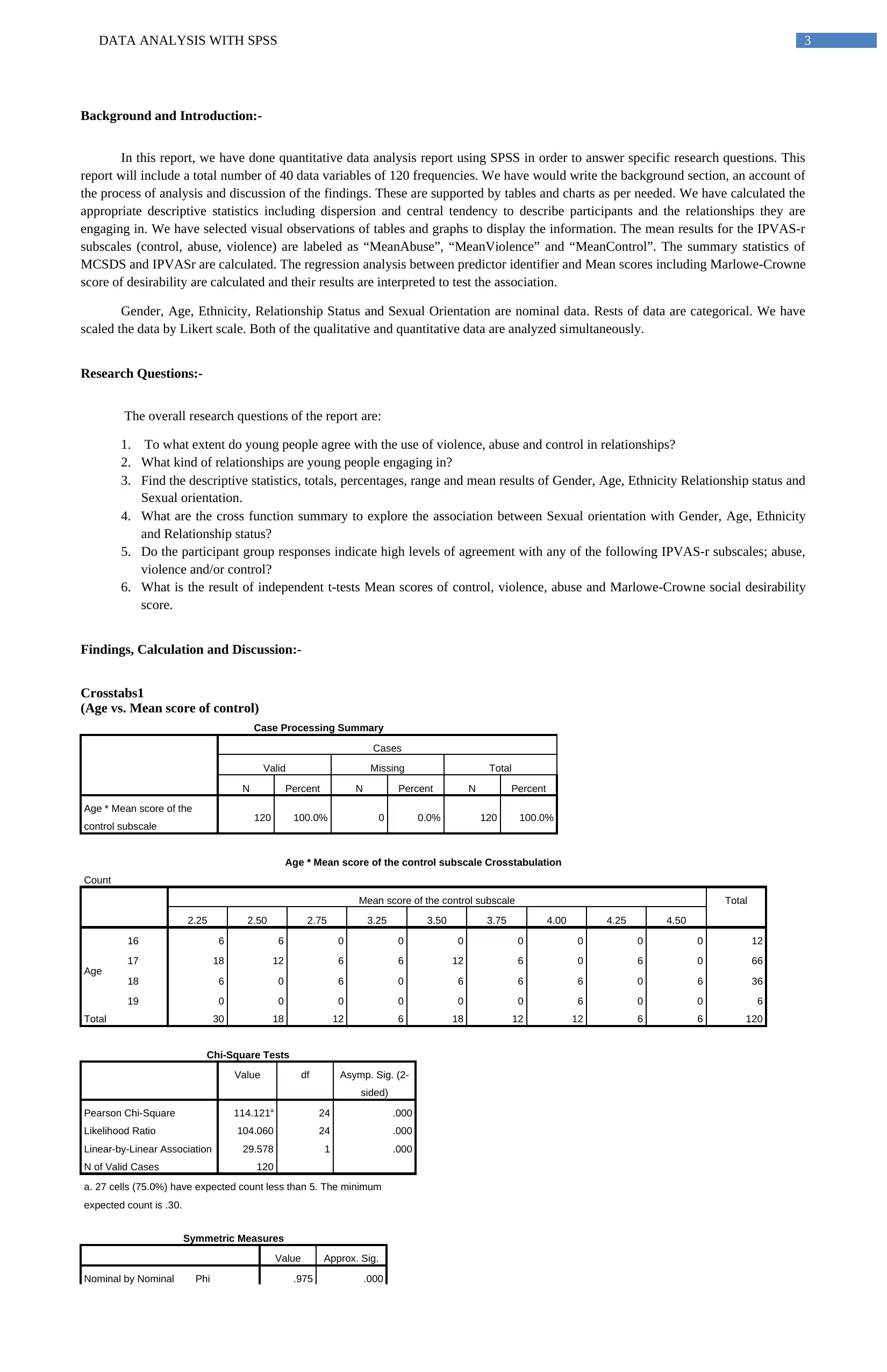
Crosstabs1
(Age vs. Mean score of control)
Case Processing Summary
Cases
Valid Missing Total
N Percent N Percent N Percent
Age * Mean score of the
control subscale 120 100.0% 0 0.0% 120 100.0%
Age * Mean score of the control subscale Crosstabulation
Count
Mean score of the control subscale Total
2.25 2.50 2.75 3.25 3.50 3.75 4.00 4.25 4.50
Age
16 6 6 0 0 0 0 0 0 0 12
17 18 12 6 6 12 6 0 6 0 66
18 6 0 6 0 6 6 6 0 6 36
19 0 0 0 0 0 0 6 0 0 6
Total 30 18 12 6 18 12 12 6 6 120
Chi-Square Tests
Value df Asymp. Sig. (2-
sided)
Pearson Chi-Square 114.121a 24 .000
Likelihood Ratio 104.060 24 .000
Linear-by-Linear Association 29.578 1 .000
N of Valid Cases 120
a. 27 cells (75.0%) have expected count less than 5. The minimum
expected count is .30.
Symmetric Measures
Value Approx. Sig.
Nominal by Nominal Phi .975 .000
Background and Introduction:-
In this report, we have done quantitative data analysis report using SPSS in order to answer specific research questions. This
report will include a total number of 40 data variables of 120 frequencies. We have would write the background section, an account of
the process of analysis and discussion of the findings. These are supported by tables and charts as per needed. We have calculated the
appropriate descriptive statistics including dispersion and central tendency to describe participants and the relationships they are
engaging in. We have selected visual observations of tables and graphs to display the information. The mean results for the IPVAS-r
subscales (control, abuse, violence) are labeled as “MeanAbuse”, “MeanViolence” and “MeanControl”. The summary statistics of
MCSDS and IPVASr are calculated. The regression analysis between predictor identifier and Mean scores including Marlowe-Crowne
score of desirability are calculated and their results are interpreted to test the association.
Gender, Age, Ethnicity, Relationship Status and Sexual Orientation are nominal data. Rests of data are categorical. We have
scaled the data by Likert scale. Both of the qualitative and quantitative data are analyzed simultaneously.
Research Questions:-
The overall research questions of the report are:
1. To what extent do young people agree with the use of violence, abuse and control in relationships?
2. What kind of relationships are young people engaging in?
3. Find the descriptive statistics, totals, percentages, range and mean results of Gender, Age, Ethnicity Relationship status and
Sexual orientation.
4. What are the cross function summary to explore the association between Sexual orientation with Gender, Age, Ethnicity
and Relationship status?
5. Do the participant group responses indicate high levels of agreement with any of the following IPVAS-r subscales; abuse,
violence and/or control?
6. What is the result of independent t-tests Mean scores of control, violence, abuse and Marlowe-Crowne social desirability
score.
Findings, Calculation and Discussion:-
Crosstabs1
(Age vs. Mean score of control)
Case Processing Summary
Cases
Valid Missing Total
N Percent N Percent N Percent
Age * Mean score of the
control subscale 120 100.0% 0 0.0% 120 100.0%
Age * Mean score of the control subscale Crosstabulation
Count
Mean score of the control subscale Total
2.25 2.50 2.75 3.25 3.50 3.75 4.00 4.25 4.50
Age
16 6 6 0 0 0 0 0 0 0 12
17 18 12 6 6 12 6 0 6 0 66
18 6 0 6 0 6 6 6 0 6 36
19 0 0 0 0 0 0 6 0 0 6
Total 30 18 12 6 18 12 12 6 6 120
Chi-Square Tests
Value df Asymp. Sig. (2-
sided)
Pearson Chi-Square 114.121a 24 .000
Likelihood Ratio 104.060 24 .000
Linear-by-Linear Association 29.578 1 .000
N of Valid Cases 120
a. 27 cells (75.0%) have expected count less than 5. The minimum
expected count is .30.
Symmetric Measures
Value Approx. Sig.
Nominal by Nominal Phi .975 .000
Paraphrase This Document
Need a fresh take? Get an instant paraphrase of this document with our AI Paraphraser
DATA ANALYSIS WITH SPSS 4
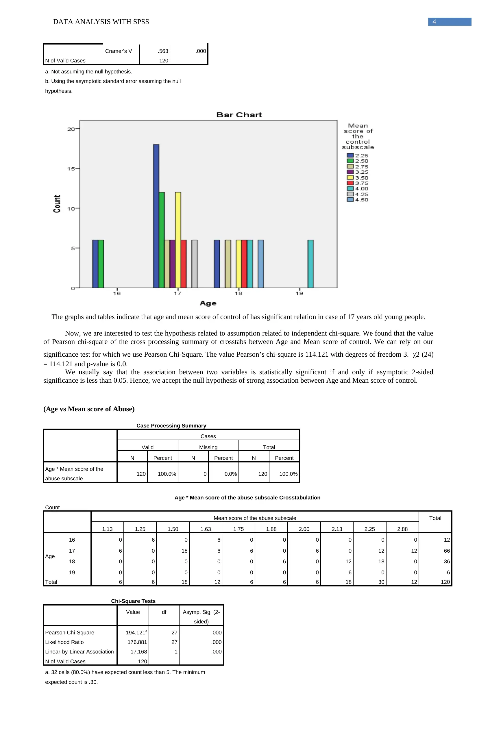
Cramer's V .563 .000
N of Valid Cases 120
a. Not assuming the null hypothesis.
b. Using the asymptotic standard error assuming the null
hypothesis.
The graphs and tables indicate that age and mean score of control of has significant relation in case of 17 years old young people.
Now, we are interested to test the hypothesis related to assumption related to independent chi-square. We found that the value
of Pearson chi-square of the cross processing summary of crosstabs between Age and Mean score of control. We can rely on our
significance test for which we use Pearson Chi-Square. The value Pearson’s chi-square is 114.121 with degrees of freedom 3. χ2 (24)
= 114.121 and p-value is 0.0.
We usually say that the association between two variables is statistically significant if and only if asymptotic 2-sided
significance is less than 0.05. Hence, we accept the null hypothesis of strong association between Age and Mean score of control.
(Age vs Mean score of Abuse)
Case Processing Summary
Cases
Valid Missing Total
N Percent N Percent N Percent
Age * Mean score of the
abuse subscale 120 100.0% 0 0.0% 120 100.0%
Age * Mean score of the abuse subscale Crosstabulation
Count
Mean score of the abuse subscale Total
1.13 1.25 1.50 1.63 1.75 1.88 2.00 2.13 2.25 2.88
Age
16 0 6 0 6 0 0 0 0 0 0 12
17 6 0 18 6 6 0 6 0 12 12 66
18 0 0 0 0 0 6 0 12 18 0 36
19 0 0 0 0 0 0 0 6 0 0 6
Total 6 6 18 12 6 6 6 18 30 12 120
Chi-Square Tests
Value df Asymp. Sig. (2-
sided)
Pearson Chi-Square 194.121a 27 .000
Likelihood Ratio 176.881 27 .000
Linear-by-Linear Association 17.168 1 .000
N of Valid Cases 120
a. 32 cells (80.0%) have expected count less than 5. The minimum
expected count is .30.
DATA ANALYSIS WITH SPSS 5
Symmetric Measures
Value Approx. Sig.
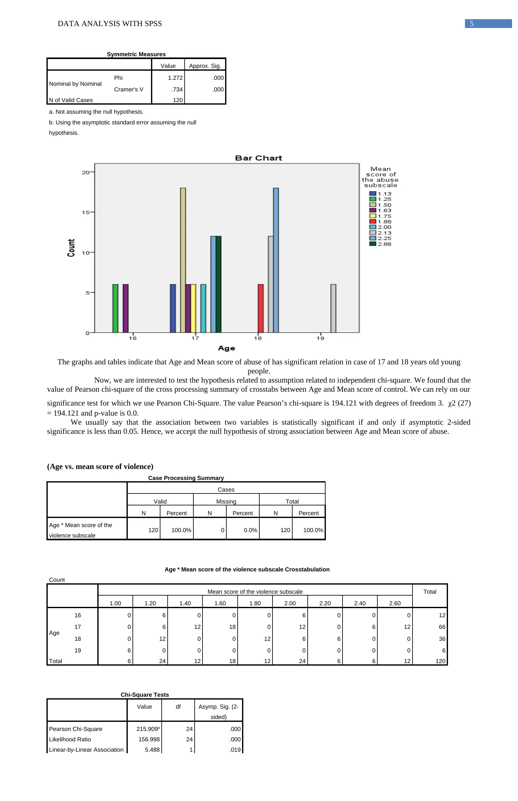
Nominal by Nominal Phi 1.272 .000
Cramer's V .734 .000
N of Valid Cases 120
a. Not assuming the null hypothesis.
b. Using the asymptotic standard error assuming the null
hypothesis.
The graphs and tables indicate that Age and Mean score of abuse of has significant relation in case of 17 and 18 years old young
people.
Now, we are interested to test the hypothesis related to assumption related to independent chi-square. We found that the
value of Pearson chi-square of the cross processing summary of crosstabs between Age and Mean score of control. We can rely on our
significance test for which we use Pearson Chi-Square. The value Pearson’s chi-square is 194.121 with degrees of freedom 3. χ2 (27)
= 194.121 and p-value is 0.0.
We usually say that the association between two variables is statistically significant if and only if asymptotic 2-sided
significance is less than 0.05. Hence, we accept the null hypothesis of strong association between Age and Mean score of abuse.
(Age vs. mean score of violence)
Case Processing Summary
Cases
Valid Missing Total
N Percent N Percent N Percent
Age * Mean score of the
violence subscale 120 100.0% 0 0.0% 120 100.0%
Age * Mean score of the violence subscale Crosstabulation
Count
Mean score of the violence subscale Total
1.00 1.20 1.40 1.60 1.80 2.00 2.20 2.40 2.60
Age
16 0 6 0 0 0 6 0 0 0 12
17 0 6 12 18 0 12 0 6 12 66
18 0 12 0 0 12 6 6 0 0 36
19 6 0 0 0 0 0 0 0 0 6
Total 6 24 12 18 12 24 6 6 12 120
Chi-Square Tests
Value df Asymp. Sig. (2-
sided)
Pearson Chi-Square 215.909a 24 .000
Likelihood Ratio 156.998 24 .000
Linear-by-Linear Association 5.488 1 .019
Symmetric Measures
Value Approx. Sig.
Nominal by Nominal Phi 1.272 .000
Cramer's V .734 .000
N of Valid Cases 120
a. Not assuming the null hypothesis.
b. Using the asymptotic standard error assuming the null
hypothesis.
The graphs and tables indicate that Age and Mean score of abuse of has significant relation in case of 17 and 18 years old young
people.
Now, we are interested to test the hypothesis related to assumption related to independent chi-square. We found that the
value of Pearson chi-square of the cross processing summary of crosstabs between Age and Mean score of control. We can rely on our
significance test for which we use Pearson Chi-Square. The value Pearson’s chi-square is 194.121 with degrees of freedom 3. χ2 (27)
= 194.121 and p-value is 0.0.
We usually say that the association between two variables is statistically significant if and only if asymptotic 2-sided
significance is less than 0.05. Hence, we accept the null hypothesis of strong association between Age and Mean score of abuse.
(Age vs. mean score of violence)
Case Processing Summary
Cases
Valid Missing Total
N Percent N Percent N Percent
Age * Mean score of the
violence subscale 120 100.0% 0 0.0% 120 100.0%
Age * Mean score of the violence subscale Crosstabulation
Count
Mean score of the violence subscale Total
1.00 1.20 1.40 1.60 1.80 2.00 2.20 2.40 2.60
Age
16 0 6 0 0 0 6 0 0 0 12
17 0 6 12 18 0 12 0 6 12 66
18 0 12 0 0 12 6 6 0 0 36
19 6 0 0 0 0 0 0 0 0 6
Total 6 24 12 18 12 24 6 6 12 120
Chi-Square Tests
Value df Asymp. Sig. (2-
sided)
Pearson Chi-Square 215.909a 24 .000
Likelihood Ratio 156.998 24 .000
Linear-by-Linear Association 5.488 1 .019
⊘ This is a preview!⊘
Do you want full access?
Subscribe today to unlock all pages.
Trusted by 1+ million students worldwide
DATA ANALYSIS WITH SPSS 6
N of Valid Cases 120
a. 27 cells (75.0%) have expected count less than 5. The minimum
expected count is .30.
Symmetric Measures
Value Approx. Sig.
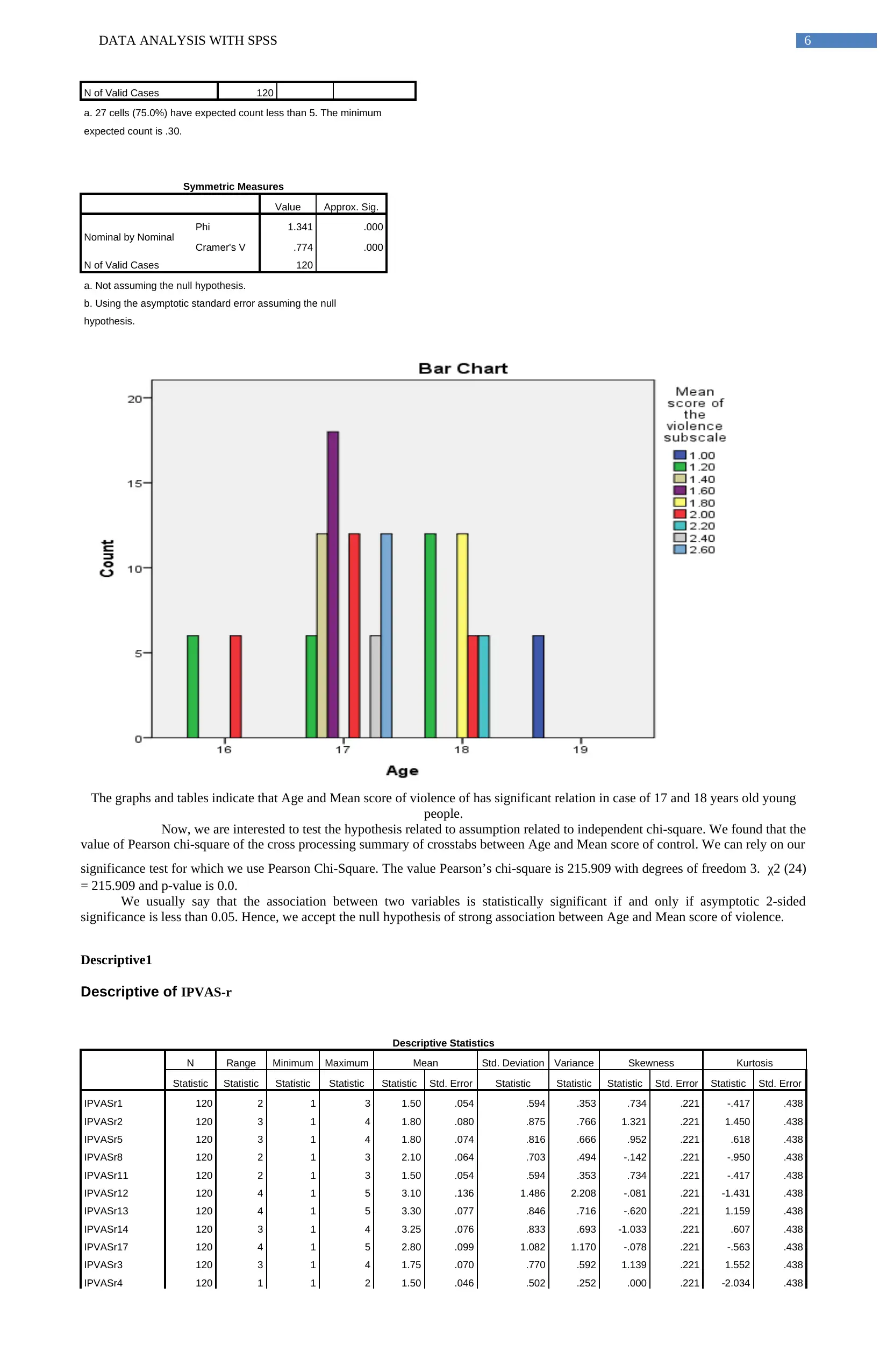
Nominal by Nominal Phi 1.341 .000
Cramer's V .774 .000
N of Valid Cases 120
a. Not assuming the null hypothesis.
b. Using the asymptotic standard error assuming the null
hypothesis.
The graphs and tables indicate that Age and Mean score of violence of has significant relation in case of 17 and 18 years old young
people.
Now, we are interested to test the hypothesis related to assumption related to independent chi-square. We found that the
value of Pearson chi-square of the cross processing summary of crosstabs between Age and Mean score of control. We can rely on our
significance test for which we use Pearson Chi-Square. The value Pearson’s chi-square is 215.909 with degrees of freedom 3. χ2 (24)
= 215.909 and p-value is 0.0.
We usually say that the association between two variables is statistically significant if and only if asymptotic 2-sided
significance is less than 0.05. Hence, we accept the null hypothesis of strong association between Age and Mean score of violence.
Descriptive1
Descriptive of IPVAS-r
Descriptive Statistics
N Range Minimum Maximum Mean Std. Deviation Variance Skewness Kurtosis
Statistic Statistic Statistic Statistic Statistic Std. Error Statistic Statistic Statistic Std. Error Statistic Std. Error
IPVASr1 120 2 1 3 1.50 .054 .594 .353 .734 .221 -.417 .438
IPVASr2 120 3 1 4 1.80 .080 .875 .766 1.321 .221 1.450 .438
IPVASr5 120 3 1 4 1.80 .074 .816 .666 .952 .221 .618 .438
IPVASr8 120 2 1 3 2.10 .064 .703 .494 -.142 .221 -.950 .438
IPVASr11 120 2 1 3 1.50 .054 .594 .353 .734 .221 -.417 .438
IPVASr12 120 4 1 5 3.10 .136 1.486 2.208 -.081 .221 -1.431 .438
IPVASr13 120 4 1 5 3.30 .077 .846 .716 -.620 .221 1.159 .438
IPVASr14 120 3 1 4 3.25 .076 .833 .693 -1.033 .221 .607 .438
IPVASr17 120 4 1 5 2.80 .099 1.082 1.170 -.078 .221 -.563 .438
IPVASr3 120 3 1 4 1.75 .070 .770 .592 1.139 .221 1.552 .438
IPVASr4 120 1 1 2 1.50 .046 .502 .252 .000 .221 -2.034 .438
N of Valid Cases 120
a. 27 cells (75.0%) have expected count less than 5. The minimum
expected count is .30.
Symmetric Measures
Value Approx. Sig.
Nominal by Nominal Phi 1.341 .000
Cramer's V .774 .000
N of Valid Cases 120
a. Not assuming the null hypothesis.
b. Using the asymptotic standard error assuming the null
hypothesis.
The graphs and tables indicate that Age and Mean score of violence of has significant relation in case of 17 and 18 years old young
people.
Now, we are interested to test the hypothesis related to assumption related to independent chi-square. We found that the
value of Pearson chi-square of the cross processing summary of crosstabs between Age and Mean score of control. We can rely on our
significance test for which we use Pearson Chi-Square. The value Pearson’s chi-square is 215.909 with degrees of freedom 3. χ2 (24)
= 215.909 and p-value is 0.0.
We usually say that the association between two variables is statistically significant if and only if asymptotic 2-sided
significance is less than 0.05. Hence, we accept the null hypothesis of strong association between Age and Mean score of violence.
Descriptive1
Descriptive of IPVAS-r
Descriptive Statistics
N Range Minimum Maximum Mean Std. Deviation Variance Skewness Kurtosis
Statistic Statistic Statistic Statistic Statistic Std. Error Statistic Statistic Statistic Std. Error Statistic Std. Error
IPVASr1 120 2 1 3 1.50 .054 .594 .353 .734 .221 -.417 .438
IPVASr2 120 3 1 4 1.80 .080 .875 .766 1.321 .221 1.450 .438
IPVASr5 120 3 1 4 1.80 .074 .816 .666 .952 .221 .618 .438
IPVASr8 120 2 1 3 2.10 .064 .703 .494 -.142 .221 -.950 .438
IPVASr11 120 2 1 3 1.50 .054 .594 .353 .734 .221 -.417 .438
IPVASr12 120 4 1 5 3.10 .136 1.486 2.208 -.081 .221 -1.431 .438
IPVASr13 120 4 1 5 3.30 .077 .846 .716 -.620 .221 1.159 .438
IPVASr14 120 3 1 4 3.25 .076 .833 .693 -1.033 .221 .607 .438
IPVASr17 120 4 1 5 2.80 .099 1.082 1.170 -.078 .221 -.563 .438
IPVASr3 120 3 1 4 1.75 .070 .770 .592 1.139 .221 1.552 .438
IPVASr4 120 1 1 2 1.50 .046 .502 .252 .000 .221 -2.034 .438
Paraphrase This Document
Need a fresh take? Get an instant paraphrase of this document with our AI Paraphraser
DATA ANALYSIS WITH SPSS 7
IPVASr6 120 3 1 4 1.70 .072 .784 .615 1.224 .221 1.558 .438
IPVASr7 120 3 1 4 2.40 .084 .920 .847 .300 .221 -.707 .438
IPVASr9 120 3 1 4 1.75 .070 .770 .592 1.139 .221 1.552 .438
IPVASr10 120 3 1 4 1.80 .080 .875 .766 .862 .221 -.067 .438
IPVASr15 120 3 1 4 2.20 .090 .984 .968 .556 .221 -.638 .438
IPVASr16 120 3 1 4 2.55 .079 .868 .754 .079 .221 -.667 .438
Valid N (listwise) 120
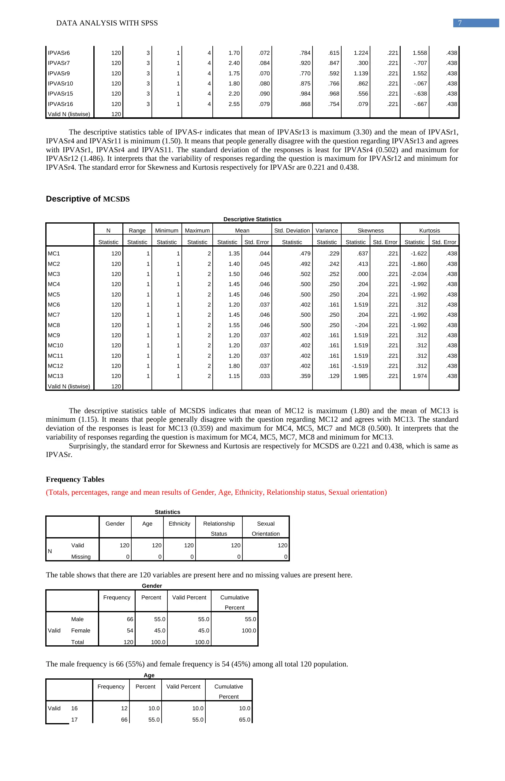
The descriptive statistics table of IPVAS-r indicates that mean of IPVASr13 is maximum (3.30) and the mean of IPVASr1,
IPVASr4 and IPVASr11 is minimum (1.50). It means that people generally disagree with the question regarding IPVASr13 and agrees
with IPVASr1, IPVASr4 and IPVAS11. The standard deviation of the responses is least for IPVASr4 (0.502) and maximum for
IPVASr12 (1.486). It interprets that the variability of responses regarding the question is maximum for IPVASr12 and minimum for
IPVASr4. The standard error for Skewness and Kurtosis respectively for IPVASr are 0.221 and 0.438.
Descriptive of MCSDS
Descriptive Statistics
N Range Minimum Maximum Mean Std. Deviation Variance Skewness Kurtosis
Statistic Statistic Statistic Statistic Statistic Std. Error Statistic Statistic Statistic Std. Error Statistic Std. Error
MC1 120 1 1 2 1.35 .044 .479 .229 .637 .221 -1.622 .438
MC2 120 1 1 2 1.40 .045 .492 .242 .413 .221 -1.860 .438
MC3 120 1 1 2 1.50 .046 .502 .252 .000 .221 -2.034 .438
MC4 120 1 1 2 1.45 .046 .500 .250 .204 .221 -1.992 .438
MC5 120 1 1 2 1.45 .046 .500 .250 .204 .221 -1.992 .438
MC6 120 1 1 2 1.20 .037 .402 .161 1.519 .221 .312 .438
MC7 120 1 1 2 1.45 .046 .500 .250 .204 .221 -1.992 .438
MC8 120 1 1 2 1.55 .046 .500 .250 -.204 .221 -1.992 .438
MC9 120 1 1 2 1.20 .037 .402 .161 1.519 .221 .312 .438
MC10 120 1 1 2 1.20 .037 .402 .161 1.519 .221 .312 .438
MC11 120 1 1 2 1.20 .037 .402 .161 1.519 .221 .312 .438
MC12 120 1 1 2 1.80 .037 .402 .161 -1.519 .221 .312 .438
MC13 120 1 1 2 1.15 .033 .359 .129 1.985 .221 1.974 .438
Valid N (listwise) 120
The descriptive statistics table of MCSDS indicates that mean of MC12 is maximum (1.80) and the mean of MC13 is
minimum (1.15). It means that people generally disagree with the question regarding MC12 and agrees with MC13. The standard
deviation of the responses is least for MC13 (0.359) and maximum for MC4, MC5, MC7 and MC8 (0.500). It interprets that the
variability of responses regarding the question is maximum for MC4, MC5, MC7, MC8 and minimum for MC13.
Surprisingly, the standard error for Skewness and Kurtosis are respectively for MCSDS are 0.221 and 0.438, which is same as
IPVASr.
Frequency Tables
(Totals, percentages, range and mean results of Gender, Age, Ethnicity, Relationship status, Sexual orientation)
Statistics
Gender Age Ethnicity Relationship
Status
Sexual
Orientation
N Valid 120 120 120 120 120
Missing 0 0 0 0 0
The table shows that there are 120 variables are present here and no missing values are present here.
Gender
Frequency Percent Valid Percent Cumulative
Percent
Valid
Male 66 55.0 55.0 55.0
Female 54 45.0 45.0 100.0
Total 120 100.0 100.0
The male frequency is 66 (55%) and female frequency is 54 (45%) among all total 120 population.
Age
Frequency Percent Valid Percent Cumulative
Percent
Valid 16 12 10.0 10.0 10.0
17 66 55.0 55.0 65.0
IPVASr6 120 3 1 4 1.70 .072 .784 .615 1.224 .221 1.558 .438
IPVASr7 120 3 1 4 2.40 .084 .920 .847 .300 .221 -.707 .438
IPVASr9 120 3 1 4 1.75 .070 .770 .592 1.139 .221 1.552 .438
IPVASr10 120 3 1 4 1.80 .080 .875 .766 .862 .221 -.067 .438
IPVASr15 120 3 1 4 2.20 .090 .984 .968 .556 .221 -.638 .438
IPVASr16 120 3 1 4 2.55 .079 .868 .754 .079 .221 -.667 .438
Valid N (listwise) 120
The descriptive statistics table of IPVAS-r indicates that mean of IPVASr13 is maximum (3.30) and the mean of IPVASr1,
IPVASr4 and IPVASr11 is minimum (1.50). It means that people generally disagree with the question regarding IPVASr13 and agrees
with IPVASr1, IPVASr4 and IPVAS11. The standard deviation of the responses is least for IPVASr4 (0.502) and maximum for
IPVASr12 (1.486). It interprets that the variability of responses regarding the question is maximum for IPVASr12 and minimum for
IPVASr4. The standard error for Skewness and Kurtosis respectively for IPVASr are 0.221 and 0.438.
Descriptive of MCSDS
Descriptive Statistics
N Range Minimum Maximum Mean Std. Deviation Variance Skewness Kurtosis
Statistic Statistic Statistic Statistic Statistic Std. Error Statistic Statistic Statistic Std. Error Statistic Std. Error
MC1 120 1 1 2 1.35 .044 .479 .229 .637 .221 -1.622 .438
MC2 120 1 1 2 1.40 .045 .492 .242 .413 .221 -1.860 .438
MC3 120 1 1 2 1.50 .046 .502 .252 .000 .221 -2.034 .438
MC4 120 1 1 2 1.45 .046 .500 .250 .204 .221 -1.992 .438
MC5 120 1 1 2 1.45 .046 .500 .250 .204 .221 -1.992 .438
MC6 120 1 1 2 1.20 .037 .402 .161 1.519 .221 .312 .438
MC7 120 1 1 2 1.45 .046 .500 .250 .204 .221 -1.992 .438
MC8 120 1 1 2 1.55 .046 .500 .250 -.204 .221 -1.992 .438
MC9 120 1 1 2 1.20 .037 .402 .161 1.519 .221 .312 .438
MC10 120 1 1 2 1.20 .037 .402 .161 1.519 .221 .312 .438
MC11 120 1 1 2 1.20 .037 .402 .161 1.519 .221 .312 .438
MC12 120 1 1 2 1.80 .037 .402 .161 -1.519 .221 .312 .438
MC13 120 1 1 2 1.15 .033 .359 .129 1.985 .221 1.974 .438
Valid N (listwise) 120
The descriptive statistics table of MCSDS indicates that mean of MC12 is maximum (1.80) and the mean of MC13 is
minimum (1.15). It means that people generally disagree with the question regarding MC12 and agrees with MC13. The standard
deviation of the responses is least for MC13 (0.359) and maximum for MC4, MC5, MC7 and MC8 (0.500). It interprets that the
variability of responses regarding the question is maximum for MC4, MC5, MC7, MC8 and minimum for MC13.
Surprisingly, the standard error for Skewness and Kurtosis are respectively for MCSDS are 0.221 and 0.438, which is same as
IPVASr.
Frequency Tables
(Totals, percentages, range and mean results of Gender, Age, Ethnicity, Relationship status, Sexual orientation)
Statistics
Gender Age Ethnicity Relationship
Status
Sexual
Orientation
N Valid 120 120 120 120 120
Missing 0 0 0 0 0
The table shows that there are 120 variables are present here and no missing values are present here.
Gender
Frequency Percent Valid Percent Cumulative
Percent
Valid
Male 66 55.0 55.0 55.0
Female 54 45.0 45.0 100.0
Total 120 100.0 100.0
The male frequency is 66 (55%) and female frequency is 54 (45%) among all total 120 population.
Age
Frequency Percent Valid Percent Cumulative
Percent
Valid 16 12 10.0 10.0 10.0
17 66 55.0 55.0 65.0
DATA ANALYSIS WITH SPSS 8
18 36 30.0 30.0 95.0
19 6 5.0 5.0 100.0
Total 120 100.0 100.0
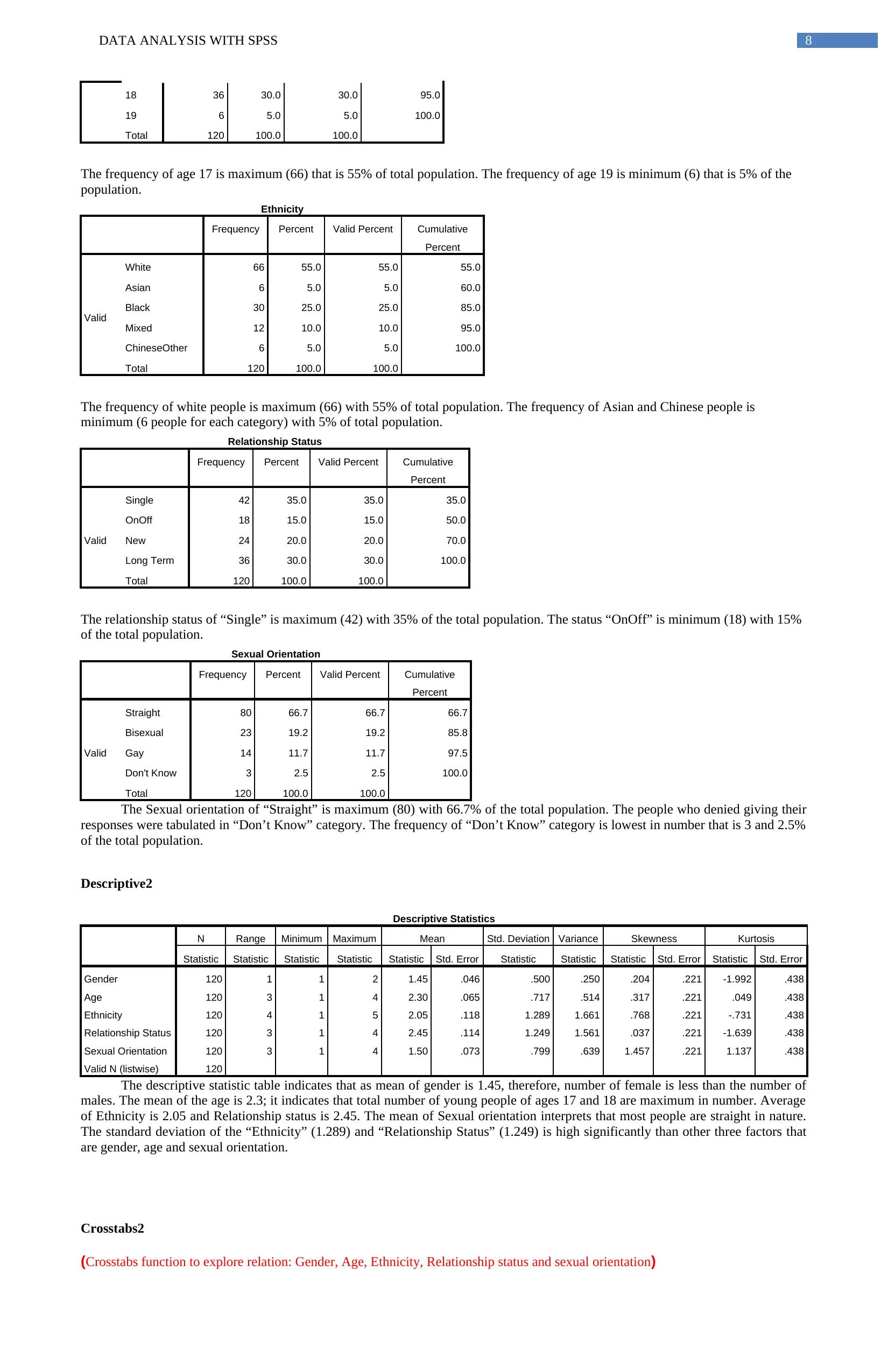
The frequency of age 17 is maximum (66) that is 55% of total population. The frequency of age 19 is minimum (6) that is 5% of the
population.
Ethnicity
Frequency Percent Valid Percent Cumulative
Percent
Valid
White 66 55.0 55.0 55.0
Asian 6 5.0 5.0 60.0
Black 30 25.0 25.0 85.0
Mixed 12 10.0 10.0 95.0
ChineseOther 6 5.0 5.0 100.0
Total 120 100.0 100.0
The frequency of white people is maximum (66) with 55% of total population. The frequency of Asian and Chinese people is
minimum (6 people for each category) with 5% of total population.
Relationship Status
Frequency Percent Valid Percent Cumulative
Percent
Valid
Single 42 35.0 35.0 35.0
OnOff 18 15.0 15.0 50.0
New 24 20.0 20.0 70.0
Long Term 36 30.0 30.0 100.0
Total 120 100.0 100.0
The relationship status of “Single” is maximum (42) with 35% of the total population. The status “OnOff” is minimum (18) with 15%
of the total population.
Sexual Orientation
Frequency Percent Valid Percent Cumulative
Percent
Valid
Straight 80 66.7 66.7 66.7
Bisexual 23 19.2 19.2 85.8
Gay 14 11.7 11.7 97.5
Don't Know 3 2.5 2.5 100.0
Total 120 100.0 100.0
The Sexual orientation of “Straight” is maximum (80) with 66.7% of the total population. The people who denied giving their
responses were tabulated in “Don’t Know” category. The frequency of “Don’t Know” category is lowest in number that is 3 and 2.5%
of the total population.
Descriptive2
Descriptive Statistics
N Range Minimum Maximum Mean Std. Deviation Variance Skewness Kurtosis
Statistic Statistic Statistic Statistic Statistic Std. Error Statistic Statistic Statistic Std. Error Statistic Std. Error
Gender 120 1 1 2 1.45 .046 .500 .250 .204 .221 -1.992 .438
Age 120 3 1 4 2.30 .065 .717 .514 .317 .221 .049 .438
Ethnicity 120 4 1 5 2.05 .118 1.289 1.661 .768 .221 -.731 .438
Relationship Status 120 3 1 4 2.45 .114 1.249 1.561 .037 .221 -1.639 .438
Sexual Orientation 120 3 1 4 1.50 .073 .799 .639 1.457 .221 1.137 .438
Valid N (listwise) 120
The descriptive statistic table indicates that as mean of gender is 1.45, therefore, number of female is less than the number of
males. The mean of the age is 2.3; it indicates that total number of young people of ages 17 and 18 are maximum in number. Average
of Ethnicity is 2.05 and Relationship status is 2.45. The mean of Sexual orientation interprets that most people are straight in nature.
The standard deviation of the “Ethnicity” (1.289) and “Relationship Status” (1.249) is high significantly than other three factors that
are gender, age and sexual orientation.
Crosstabs2
(Crosstabs function to explore relation: Gender, Age, Ethnicity, Relationship status and sexual orientation)
18 36 30.0 30.0 95.0
19 6 5.0 5.0 100.0
Total 120 100.0 100.0
The frequency of age 17 is maximum (66) that is 55% of total population. The frequency of age 19 is minimum (6) that is 5% of the
population.
Ethnicity
Frequency Percent Valid Percent Cumulative
Percent
Valid
White 66 55.0 55.0 55.0
Asian 6 5.0 5.0 60.0
Black 30 25.0 25.0 85.0
Mixed 12 10.0 10.0 95.0
ChineseOther 6 5.0 5.0 100.0
Total 120 100.0 100.0
The frequency of white people is maximum (66) with 55% of total population. The frequency of Asian and Chinese people is
minimum (6 people for each category) with 5% of total population.
Relationship Status
Frequency Percent Valid Percent Cumulative
Percent
Valid
Single 42 35.0 35.0 35.0
OnOff 18 15.0 15.0 50.0
New 24 20.0 20.0 70.0
Long Term 36 30.0 30.0 100.0
Total 120 100.0 100.0
The relationship status of “Single” is maximum (42) with 35% of the total population. The status “OnOff” is minimum (18) with 15%
of the total population.
Sexual Orientation
Frequency Percent Valid Percent Cumulative
Percent
Valid
Straight 80 66.7 66.7 66.7
Bisexual 23 19.2 19.2 85.8
Gay 14 11.7 11.7 97.5
Don't Know 3 2.5 2.5 100.0
Total 120 100.0 100.0
The Sexual orientation of “Straight” is maximum (80) with 66.7% of the total population. The people who denied giving their
responses were tabulated in “Don’t Know” category. The frequency of “Don’t Know” category is lowest in number that is 3 and 2.5%
of the total population.
Descriptive2
Descriptive Statistics
N Range Minimum Maximum Mean Std. Deviation Variance Skewness Kurtosis
Statistic Statistic Statistic Statistic Statistic Std. Error Statistic Statistic Statistic Std. Error Statistic Std. Error
Gender 120 1 1 2 1.45 .046 .500 .250 .204 .221 -1.992 .438
Age 120 3 1 4 2.30 .065 .717 .514 .317 .221 .049 .438
Ethnicity 120 4 1 5 2.05 .118 1.289 1.661 .768 .221 -.731 .438
Relationship Status 120 3 1 4 2.45 .114 1.249 1.561 .037 .221 -1.639 .438
Sexual Orientation 120 3 1 4 1.50 .073 .799 .639 1.457 .221 1.137 .438
Valid N (listwise) 120
The descriptive statistic table indicates that as mean of gender is 1.45, therefore, number of female is less than the number of
males. The mean of the age is 2.3; it indicates that total number of young people of ages 17 and 18 are maximum in number. Average
of Ethnicity is 2.05 and Relationship status is 2.45. The mean of Sexual orientation interprets that most people are straight in nature.
The standard deviation of the “Ethnicity” (1.289) and “Relationship Status” (1.249) is high significantly than other three factors that
are gender, age and sexual orientation.
Crosstabs2
(Crosstabs function to explore relation: Gender, Age, Ethnicity, Relationship status and sexual orientation)
⊘ This is a preview!⊘
Do you want full access?
Subscribe today to unlock all pages.
Trusted by 1+ million students worldwide
DATA ANALYSIS WITH SPSS 9
Case Processing Summary
Cases
Valid Missing Total
N Percent N Percent N Percent
Sexual Orientation * Gender 120 100.0% 0 0.0% 120 100.0%
Sexual Orientation * Age 120 100.0% 0 0.0% 120 100.0%
Sexual Orientation *
Ethnicity 120 100.0% 0 0.0% 120 100.0%
Sexual Orientation *
Relationship Status 120 100.0% 0 0.0% 120 100.0%
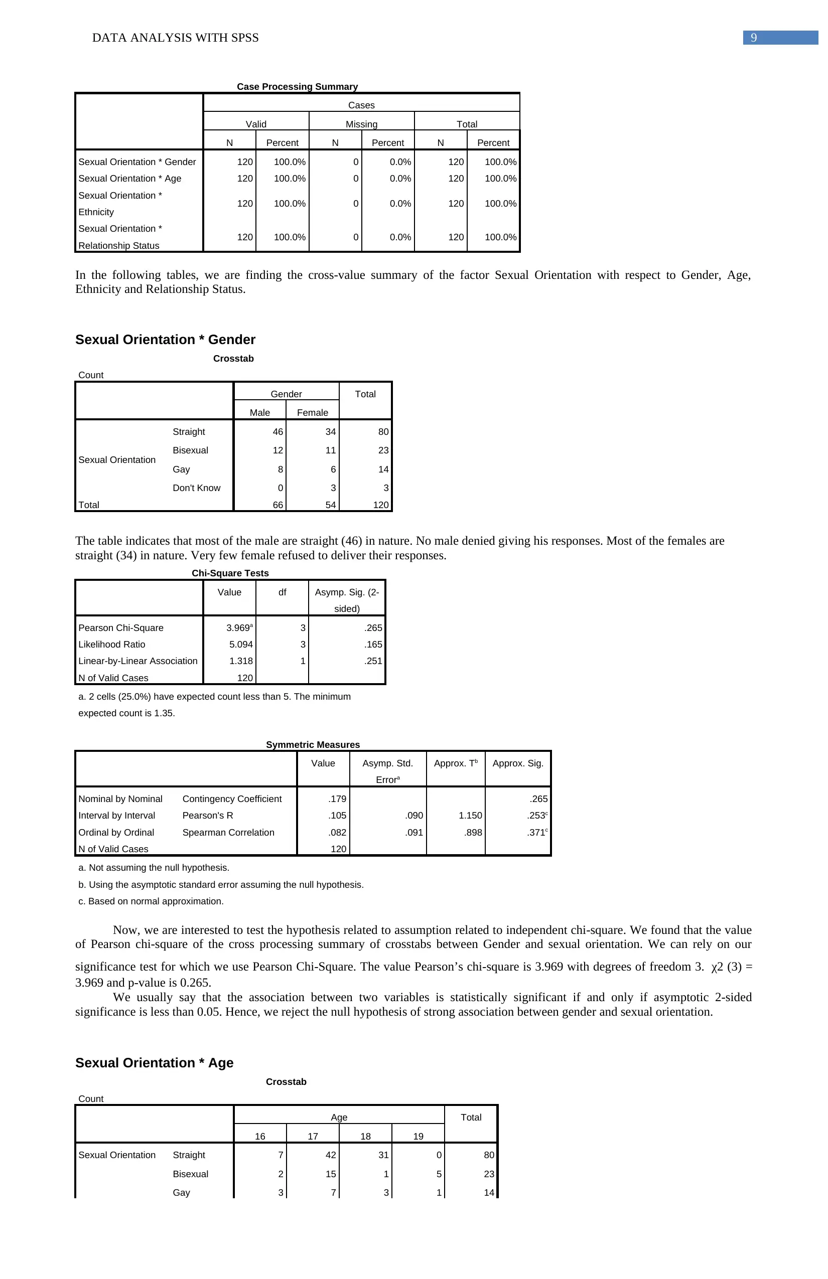
In the following tables, we are finding the cross-value summary of the factor Sexual Orientation with respect to Gender, Age,
Ethnicity and Relationship Status.
Sexual Orientation * Gender
Crosstab
Count
Gender Total
Male Female
Sexual Orientation
Straight 46 34 80
Bisexual 12 11 23
Gay 8 6 14
Don't Know 0 3 3
Total 66 54 120
The table indicates that most of the male are straight (46) in nature. No male denied giving his responses. Most of the females are
straight (34) in nature. Very few female refused to deliver their responses.
Chi-Square Tests
Value df Asymp. Sig. (2-
sided)
Pearson Chi-Square 3.969a 3 .265
Likelihood Ratio 5.094 3 .165
Linear-by-Linear Association 1.318 1 .251
N of Valid Cases 120
a. 2 cells (25.0%) have expected count less than 5. The minimum
expected count is 1.35.
Symmetric Measures
Value Asymp. Std.
Errora
Approx. Tb Approx. Sig.
Nominal by Nominal Contingency Coefficient .179 .265
Interval by Interval Pearson's R .105 .090 1.150 .253c
Ordinal by Ordinal Spearman Correlation .082 .091 .898 .371c
N of Valid Cases 120
a. Not assuming the null hypothesis.
b. Using the asymptotic standard error assuming the null hypothesis.
c. Based on normal approximation.
Now, we are interested to test the hypothesis related to assumption related to independent chi-square. We found that the value
of Pearson chi-square of the cross processing summary of crosstabs between Gender and sexual orientation. We can rely on our
significance test for which we use Pearson Chi-Square. The value Pearson’s chi-square is 3.969 with degrees of freedom 3. χ2 (3) =
3.969 and p-value is 0.265.
We usually say that the association between two variables is statistically significant if and only if asymptotic 2-sided
significance is less than 0.05. Hence, we reject the null hypothesis of strong association between gender and sexual orientation.
Sexual Orientation * Age
Crosstab
Count
Age Total
16 17 18 19
Sexual Orientation Straight 7 42 31 0 80
Bisexual 2 15 1 5 23
Gay 3 7 3 1 14
Case Processing Summary
Cases
Valid Missing Total
N Percent N Percent N Percent
Sexual Orientation * Gender 120 100.0% 0 0.0% 120 100.0%
Sexual Orientation * Age 120 100.0% 0 0.0% 120 100.0%
Sexual Orientation *
Ethnicity 120 100.0% 0 0.0% 120 100.0%
Sexual Orientation *
Relationship Status 120 100.0% 0 0.0% 120 100.0%
In the following tables, we are finding the cross-value summary of the factor Sexual Orientation with respect to Gender, Age,
Ethnicity and Relationship Status.
Sexual Orientation * Gender
Crosstab
Count
Gender Total
Male Female
Sexual Orientation
Straight 46 34 80
Bisexual 12 11 23
Gay 8 6 14
Don't Know 0 3 3
Total 66 54 120
The table indicates that most of the male are straight (46) in nature. No male denied giving his responses. Most of the females are
straight (34) in nature. Very few female refused to deliver their responses.
Chi-Square Tests
Value df Asymp. Sig. (2-
sided)
Pearson Chi-Square 3.969a 3 .265
Likelihood Ratio 5.094 3 .165
Linear-by-Linear Association 1.318 1 .251
N of Valid Cases 120
a. 2 cells (25.0%) have expected count less than 5. The minimum
expected count is 1.35.
Symmetric Measures
Value Asymp. Std.
Errora
Approx. Tb Approx. Sig.
Nominal by Nominal Contingency Coefficient .179 .265
Interval by Interval Pearson's R .105 .090 1.150 .253c
Ordinal by Ordinal Spearman Correlation .082 .091 .898 .371c
N of Valid Cases 120
a. Not assuming the null hypothesis.
b. Using the asymptotic standard error assuming the null hypothesis.
c. Based on normal approximation.
Now, we are interested to test the hypothesis related to assumption related to independent chi-square. We found that the value
of Pearson chi-square of the cross processing summary of crosstabs between Gender and sexual orientation. We can rely on our
significance test for which we use Pearson Chi-Square. The value Pearson’s chi-square is 3.969 with degrees of freedom 3. χ2 (3) =
3.969 and p-value is 0.265.
We usually say that the association between two variables is statistically significant if and only if asymptotic 2-sided
significance is less than 0.05. Hence, we reject the null hypothesis of strong association between gender and sexual orientation.
Sexual Orientation * Age
Crosstab
Count
Age Total
16 17 18 19
Sexual Orientation Straight 7 42 31 0 80
Bisexual 2 15 1 5 23
Gay 3 7 3 1 14
Paraphrase This Document
Need a fresh take? Get an instant paraphrase of this document with our AI Paraphraser
DATA ANALYSIS WITH SPSS 10
Don't Know 0 2 1 0 3
Total 12 66 36 6 120
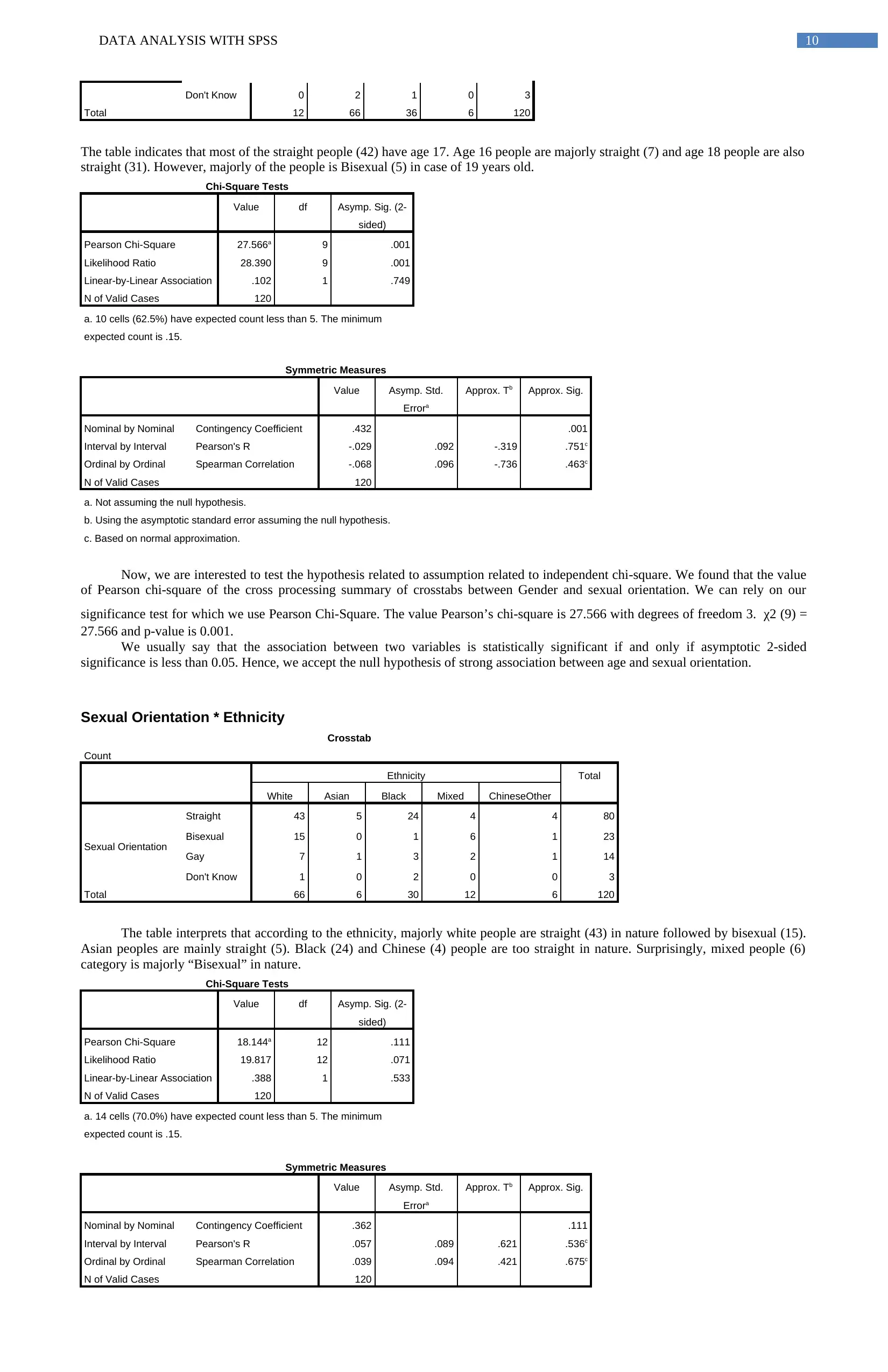
The table indicates that most of the straight people (42) have age 17. Age 16 people are majorly straight (7) and age 18 people are also
straight (31). However, majorly of the people is Bisexual (5) in case of 19 years old.
Chi-Square Tests
Value df Asymp. Sig. (2-
sided)
Pearson Chi-Square 27.566a 9 .001
Likelihood Ratio 28.390 9 .001
Linear-by-Linear Association .102 1 .749
N of Valid Cases 120
a. 10 cells (62.5%) have expected count less than 5. The minimum
expected count is .15.
Symmetric Measures
Value Asymp. Std.
Errora
Approx. Tb Approx. Sig.
Nominal by Nominal Contingency Coefficient .432 .001
Interval by Interval Pearson's R -.029 .092 -.319 .751c
Ordinal by Ordinal Spearman Correlation -.068 .096 -.736 .463c
N of Valid Cases 120
a. Not assuming the null hypothesis.
b. Using the asymptotic standard error assuming the null hypothesis.
c. Based on normal approximation.
Now, we are interested to test the hypothesis related to assumption related to independent chi-square. We found that the value
of Pearson chi-square of the cross processing summary of crosstabs between Gender and sexual orientation. We can rely on our
significance test for which we use Pearson Chi-Square. The value Pearson’s chi-square is 27.566 with degrees of freedom 3. χ2 (9) =
27.566 and p-value is 0.001.
We usually say that the association between two variables is statistically significant if and only if asymptotic 2-sided
significance is less than 0.05. Hence, we accept the null hypothesis of strong association between age and sexual orientation.
Sexual Orientation * Ethnicity
Crosstab
Count
Ethnicity Total
White Asian Black Mixed ChineseOther
Sexual Orientation
Straight 43 5 24 4 4 80
Bisexual 15 0 1 6 1 23
Gay 7 1 3 2 1 14
Don't Know 1 0 2 0 0 3
Total 66 6 30 12 6 120
The table interprets that according to the ethnicity, majorly white people are straight (43) in nature followed by bisexual (15).
Asian peoples are mainly straight (5). Black (24) and Chinese (4) people are too straight in nature. Surprisingly, mixed people (6)
category is majorly “Bisexual” in nature.
Chi-Square Tests
Value df Asymp. Sig. (2-
sided)
Pearson Chi-Square 18.144a 12 .111
Likelihood Ratio 19.817 12 .071
Linear-by-Linear Association .388 1 .533
N of Valid Cases 120
a. 14 cells (70.0%) have expected count less than 5. The minimum
expected count is .15.
Symmetric Measures
Value Asymp. Std.
Errora
Approx. Tb Approx. Sig.
Nominal by Nominal Contingency Coefficient .362 .111
Interval by Interval Pearson's R .057 .089 .621 .536c
Ordinal by Ordinal Spearman Correlation .039 .094 .421 .675c
N of Valid Cases 120
Don't Know 0 2 1 0 3
Total 12 66 36 6 120
The table indicates that most of the straight people (42) have age 17. Age 16 people are majorly straight (7) and age 18 people are also
straight (31). However, majorly of the people is Bisexual (5) in case of 19 years old.
Chi-Square Tests
Value df Asymp. Sig. (2-
sided)
Pearson Chi-Square 27.566a 9 .001
Likelihood Ratio 28.390 9 .001
Linear-by-Linear Association .102 1 .749
N of Valid Cases 120
a. 10 cells (62.5%) have expected count less than 5. The minimum
expected count is .15.
Symmetric Measures
Value Asymp. Std.
Errora
Approx. Tb Approx. Sig.
Nominal by Nominal Contingency Coefficient .432 .001
Interval by Interval Pearson's R -.029 .092 -.319 .751c
Ordinal by Ordinal Spearman Correlation -.068 .096 -.736 .463c
N of Valid Cases 120
a. Not assuming the null hypothesis.
b. Using the asymptotic standard error assuming the null hypothesis.
c. Based on normal approximation.
Now, we are interested to test the hypothesis related to assumption related to independent chi-square. We found that the value
of Pearson chi-square of the cross processing summary of crosstabs between Gender and sexual orientation. We can rely on our
significance test for which we use Pearson Chi-Square. The value Pearson’s chi-square is 27.566 with degrees of freedom 3. χ2 (9) =
27.566 and p-value is 0.001.
We usually say that the association between two variables is statistically significant if and only if asymptotic 2-sided
significance is less than 0.05. Hence, we accept the null hypothesis of strong association between age and sexual orientation.
Sexual Orientation * Ethnicity
Crosstab
Count
Ethnicity Total
White Asian Black Mixed ChineseOther
Sexual Orientation
Straight 43 5 24 4 4 80
Bisexual 15 0 1 6 1 23
Gay 7 1 3 2 1 14
Don't Know 1 0 2 0 0 3
Total 66 6 30 12 6 120
The table interprets that according to the ethnicity, majorly white people are straight (43) in nature followed by bisexual (15).
Asian peoples are mainly straight (5). Black (24) and Chinese (4) people are too straight in nature. Surprisingly, mixed people (6)
category is majorly “Bisexual” in nature.
Chi-Square Tests
Value df Asymp. Sig. (2-
sided)
Pearson Chi-Square 18.144a 12 .111
Likelihood Ratio 19.817 12 .071
Linear-by-Linear Association .388 1 .533
N of Valid Cases 120
a. 14 cells (70.0%) have expected count less than 5. The minimum
expected count is .15.
Symmetric Measures
Value Asymp. Std.
Errora
Approx. Tb Approx. Sig.
Nominal by Nominal Contingency Coefficient .362 .111
Interval by Interval Pearson's R .057 .089 .621 .536c
Ordinal by Ordinal Spearman Correlation .039 .094 .421 .675c
N of Valid Cases 120
DATA ANALYSIS WITH SPSS 11
a. Not assuming the null hypothesis.
b. Using the asymptotic standard error assuming the null hypothesis.
c. Based on normal approximation.
Now, we are interested to test the hypothesis related to assumption related to independent chi-square. We found that the value
of Pearson chi-square of the cross processing summary of crosstabs between Gender and sexual orientation. We can rely on our
significance test for which we use Pearson Chi-Square. The value Pearson’s chi-square is 18.144 with degrees of freedom 3. χ2 (12) =
18.144 and p-value is 0.111.
We usually say that the association between two variables is statistically significant if and only if asymptotic 2-sided
significance is less than 0.05. Hence, we reject the null hypothesis of strong association between Ethnicity and sexual orientation.
Sexual Orientation * Relationship Status
Crosstab
Count
Relationship Status Total
Single OnOff New Long Term
Sexual Orientation
Straight 30 14 17 19 80
Bisexual 8 1 2 12 23
Gay 3 3 4 4 14
Don't Know 1 0 1 1 3
Total 42 18 24 36 120
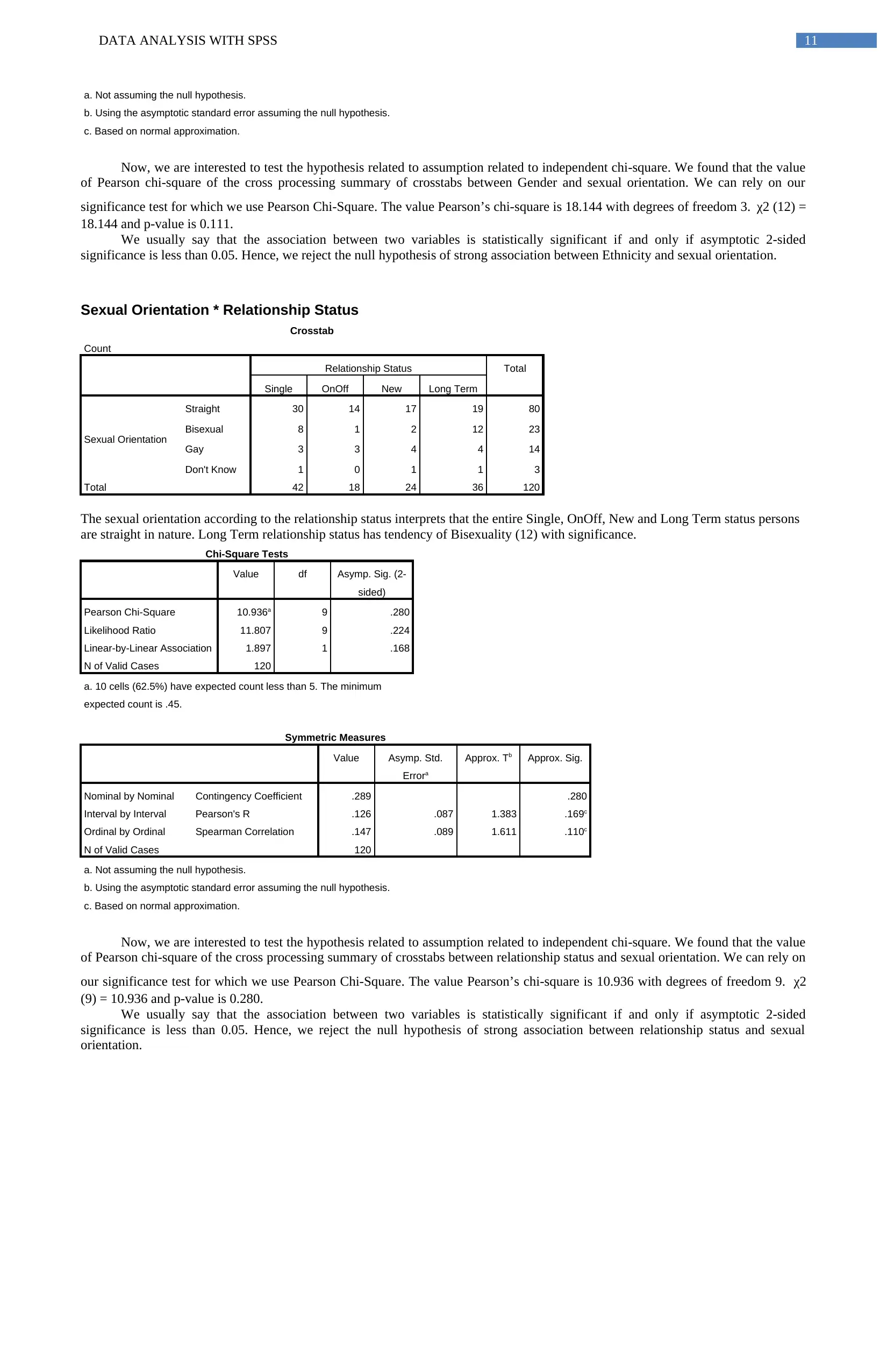
The sexual orientation according to the relationship status interprets that the entire Single, OnOff, New and Long Term status persons
are straight in nature. Long Term relationship status has tendency of Bisexuality (12) with significance.
Chi-Square Tests
Value df Asymp. Sig. (2-
sided)
Pearson Chi-Square 10.936a 9 .280
Likelihood Ratio 11.807 9 .224
Linear-by-Linear Association 1.897 1 .168
N of Valid Cases 120
a. 10 cells (62.5%) have expected count less than 5. The minimum
expected count is .45.
Symmetric Measures
Value Asymp. Std.
Errora
Approx. Tb Approx. Sig.
Nominal by Nominal Contingency Coefficient .289 .280
Interval by Interval Pearson's R .126 .087 1.383 .169c
Ordinal by Ordinal Spearman Correlation .147 .089 1.611 .110c
N of Valid Cases 120
a. Not assuming the null hypothesis.
b. Using the asymptotic standard error assuming the null hypothesis.
c. Based on normal approximation.
Now, we are interested to test the hypothesis related to assumption related to independent chi-square. We found that the value
of Pearson chi-square of the cross processing summary of crosstabs between relationship status and sexual orientation. We can rely on
our significance test for which we use Pearson Chi-Square. The value Pearson’s chi-square is 10.936 with degrees of freedom 9. χ2
(9) = 10.936 and p-value is 0.280.
We usually say that the association between two variables is statistically significant if and only if asymptotic 2-sided
significance is less than 0.05. Hence, we reject the null hypothesis of strong association between relationship status and sexual
orientation.
a. Not assuming the null hypothesis.
b. Using the asymptotic standard error assuming the null hypothesis.
c. Based on normal approximation.
Now, we are interested to test the hypothesis related to assumption related to independent chi-square. We found that the value
of Pearson chi-square of the cross processing summary of crosstabs between Gender and sexual orientation. We can rely on our
significance test for which we use Pearson Chi-Square. The value Pearson’s chi-square is 18.144 with degrees of freedom 3. χ2 (12) =
18.144 and p-value is 0.111.
We usually say that the association between two variables is statistically significant if and only if asymptotic 2-sided
significance is less than 0.05. Hence, we reject the null hypothesis of strong association between Ethnicity and sexual orientation.
Sexual Orientation * Relationship Status
Crosstab
Count
Relationship Status Total
Single OnOff New Long Term
Sexual Orientation
Straight 30 14 17 19 80
Bisexual 8 1 2 12 23
Gay 3 3 4 4 14
Don't Know 1 0 1 1 3
Total 42 18 24 36 120
The sexual orientation according to the relationship status interprets that the entire Single, OnOff, New and Long Term status persons
are straight in nature. Long Term relationship status has tendency of Bisexuality (12) with significance.
Chi-Square Tests
Value df Asymp. Sig. (2-
sided)
Pearson Chi-Square 10.936a 9 .280
Likelihood Ratio 11.807 9 .224
Linear-by-Linear Association 1.897 1 .168
N of Valid Cases 120
a. 10 cells (62.5%) have expected count less than 5. The minimum
expected count is .45.
Symmetric Measures
Value Asymp. Std.
Errora
Approx. Tb Approx. Sig.
Nominal by Nominal Contingency Coefficient .289 .280
Interval by Interval Pearson's R .126 .087 1.383 .169c
Ordinal by Ordinal Spearman Correlation .147 .089 1.611 .110c
N of Valid Cases 120
a. Not assuming the null hypothesis.
b. Using the asymptotic standard error assuming the null hypothesis.
c. Based on normal approximation.
Now, we are interested to test the hypothesis related to assumption related to independent chi-square. We found that the value
of Pearson chi-square of the cross processing summary of crosstabs between relationship status and sexual orientation. We can rely on
our significance test for which we use Pearson Chi-Square. The value Pearson’s chi-square is 10.936 with degrees of freedom 9. χ2
(9) = 10.936 and p-value is 0.280.
We usually say that the association between two variables is statistically significant if and only if asymptotic 2-sided
significance is less than 0.05. Hence, we reject the null hypothesis of strong association between relationship status and sexual
orientation.
⊘ This is a preview!⊘
Do you want full access?
Subscribe today to unlock all pages.
Trusted by 1+ million students worldwide
1 out of 19
Related Documents


Your All-in-One AI-Powered Toolkit for Academic Success.
+13062052269
info@desklib.com
Available 24*7 on WhatsApp / Email
![[object Object]](/_next/static/media/star-bottom.7253800d.svg)
Unlock your academic potential
Copyright © 2020–2026 A2Z Services. All Rights Reserved. Developed and managed by ZUCOL.